Related Plugins and Tags

QGIS Planet

Movement data in GIS #20: Trajectools v1 released!

In previous posts, I already wrote about Trajectools and some of the functionality it provides to QGIS Processing including:

There are also tools to compute heading and speed which I only talked about on Twitter.

Trajectools is now available from the QGIS plugin repository.

The plugin includes sample data from MarineCadastre downloads and the Geolife project.

Under the hood, Trajectools depends on GeoPandas!

If you are on Windows, here’s how to install GeoPandas for OSGeo4W:

  1. OSGeo4W installer: install python3-pip
  2. Environment variables: add GDAL_VERSION = 2.3.2 (or whichever version your OSGeo4W installation currently includes)
  3. OSGeo4W shell: call C:\OSGeo4W64\bin\py3_env.bat
  4. OSGeo4W shell: pip3 install geopandas (this will error at fiona)
  5. From https://www.lfd.uci.edu/~gohlke/pythonlibs/#fiona: download Fiona-1.7.13-cp37-cp37m-win_amd64.whl
  6. OSGeo4W shell: pip3 install path-to-download\Fiona-1.7.13-cp37-cp37m-win_amd64.whl
  7. OSGeo4W shell: pip3 install geopandas
  8. (optionally) From https://www.lfd.uci.edu/~gohlke/pythonlibs/#rtree: download Rtree-0.8.3-cp37-cp37m-win_amd64.whl and pip3 install it

If you want to use this functionality outside of QGIS, head over to my movingpandas project!

Call for testing: GRASS GIS with Python 3

Please help us testing the Python3 support in the yet unreleased GRASS GIS trunk (i.e., version “grass77” which will be released as “grass78” in the near future).

1. Why Python 3?

Python 2 is end-of-life (EOL); the current Python 2.7 will retire in 11 months from today (see https://pythonclock.org). We want to follow the “Moving to require Python 3” and complete the change to Python 3. And we need a broader community testing.

2. Download and test!

Packages are available at time:

3. Instructions for testing

4. Problems found? Please report them to us

Problems and bugs can be reported in the GRASS GIS trac. Code changes are welcome!

Thanks for testing grass77!

The post Call for testing: GRASS GIS with Python 3 appeared first on GFOSS Blog | GRASS GIS and OSGeo News.

Dealing with delayed measurements in (Geo)Pandas

Yesterday, I learned about a cool use case in data-driven agriculture that requires dealing with delayed measurements. As Bert mentions, for example, potatoes end up in the machines and are counted a few seconds after they’re actually taken out of the ground:

Therefore, in order to accurately map yield, we need to take this temporal offset into account.

We need to make sure that time and location stay untouched, but need to shift the potato count value. To support this use case, I’ve implemented apply_offset_seconds() for trajectories in movingpandas:

    def apply_offset_seconds(self, column, offset):
        self.df[column] = self.df[column].shift(offset, freq='1s')

The following test illustrates its use: you can see how the value column is shifted by 120 second. Geometry and time remain unchanged but the value column is shifted accordingly. In this test, we look at the row with index 2 which we access using iloc[2]:

    def test_offset_seconds(self):
        df = pd.DataFrame([
            {'geometry': Point(0, 0), 't': datetime(2018, 1, 1, 12, 0, 0), 'value': 1},
            {'geometry': Point(-6, 10), 't': datetime(2018, 1, 1, 12, 1, 0), 'value': 2},
            {'geometry': Point(6, 6), 't': datetime(2018, 1, 1, 12, 2, 0), 'value': 3},
            {'geometry': Point(6, 12), 't': datetime(2018, 1, 1, 12, 3, 0), 'value':4},
            {'geometry': Point(6, 18), 't': datetime(2018, 1, 1, 12, 4, 0), 'value':5}
        ]).set_index('t')
        geo_df = GeoDataFrame(df, crs={'init': '31256'})
        traj = Trajectory(1, geo_df)
        traj.apply_offset_seconds('value', -120)
        self.assertEqual(traj.df.iloc[2].value, 5)
        self.assertEqual(traj.df.iloc[2].geometry, Point(6, 6))

From CSV to GeoDataFrame in two lines

Pandas is great for data munging and with the help of GeoPandas, these capabilities expand into the spatial realm.

With just two lines, it’s quick and easy to transform a plain headerless CSV file into a GeoDataFrame. (If your CSV is nice and already contains a header, you can skip the header=None and names=FILE_HEADER parameters.)

usecols=USE_COLS is also optional and allows us to specify that we only want to use a subset of the columns available in the CSV.

After the obligatory imports and setting of variables, all we need to do is read the CSV into a regular DataFrame and then construct a GeoDataFrame.

import pandas as pd
from geopandas import GeoDataFrame
from shapely.geometry import Point

FILE_NAME = "/temp/your.csv"
FILE_HEADER = ['a', 'b', 'c', 'd', 'e', 'x', 'y']
USE_COLS = ['a', 'x', 'y']

df = pd.read_csv(
    FILE_NAME, delimiter=";", header=None,
    names=FILE_HEADER, usecols=USE_COLS)
gdf = GeoDataFrame(
    df.drop(['x', 'y'], axis=1),
    crs={'init': 'epsg:4326'},
    geometry=[Point(xy) for xy in zip(df.x, df.y)])

It’s also possible to create the point objects using a lambda function as shown by weiji14 on GIS.SE.

Movement data in GIS #21: new interactive notebook to get started with MovingPandas

MovingPandas is my attempt to provide a pure Python solution for trajectory data handling in GIS. MovingPandas provides trajectory classes and functions built on top of GeoPandas. 

To lower the entry barrier to getting started with MovingPandas, there’s now an interactive iPython notebook hosted on MyBinder. This notebook provides all the necessary imports and demonstrates how to create a Trajectory object.

Launch MyBinder for MovingPandas to get started!

PyQGIS101 part 10 published!

PyQGIS 101: Introduction to QGIS Python programming for non-programmers has now reached the part 10 milestone!

Beyond the obligatory Hello world! example, the contents so far include:

If you’ve been thinking about learning Python programming, but never got around to actually start doing it, give PyQGIS101 a try.

I’d like to thank everyone who has already provided feedback to the exercises. Every comment is important to help me understand the pain points of learning Python for QGIS.

I recently read an article – unfortunately I forgot to bookmark it and cannot locate it anymore – that described the problems with learning to program very well: in the beginning, it’s rather slow going, you don’t know the right terminology and therefore don’t know what to google for when you run into issues. But there comes this point, when you finally get it, when the terminology becomes clearer, when you start thinking “that might work” and it actually does! I hope that PyQGIS101 will be a help along the way.

Movement data in GIS #18: creating evaluation data for trajectory predictions

We’ve seen a lot of explorative movement data analysis in the Movement data in GIS series so far. Beyond exploration, predictive analysis is another major topic in movement data analysis. One of the most obvious movement prediction use cases is trajectory prediction, i.e. trying to predict where a moving object will be in the future. The two main categories of trajectory prediction methods I see are those that try to predict the actual path that a moving object will take versus those that only try to predict the next destination.

Today, I want to focus on prediction methods that predict the path that a moving object is going to take. There are many different approaches from simple linear prediction to very sophisticated application-dependent methods. Regardless of the prediction method though, there is the question of how to evaluate the prediction results when these methods are applied to real-life data.

As long as we work with nice, densely, and regularly updated movement data, extracting evaluation samples is rather straightforward. To predict future movement, we need some information about past movement. Based on that past movement, we can then try to predict future positions. For example, given a trajectory that is twenty minutes long, we can extract a sample that provides five minutes of past movement, as well as the actually observed position five minutes into the future:

But what if the trajectory is irregularly updated? Do we interpolate the positions at the desired five minute timestamps? Do we try to shift the sample until – by chance – we find a section along the trajectory where the updates match our desired pattern? What if location timestamps include seconds or milliseconds and we therefore cannot find exact matches? Should we introduce a tolerance parameter that would allow us to match locations with approximately the same timestamp?

Depending on the duration of observation gaps in our trajectory, it might not be a good idea to simply interpolate locations since these interpolated locations could systematically bias our evaluation. Therefore, the safest approach may be to shift the sample pattern along the trajectory until a close match (within the specified tolerance) is found. This approach is now implemented in MovingPandas’ TrajectorySampler.

def test_sample_irregular_updates(self):
    df = pd.DataFrame([
        {'geometry':Point(0,0), 't':datetime(2018,1,1,12,0,1)},
        {'geometry':Point(0,3), 't':datetime(2018,1,1,12,3,2)},
        {'geometry':Point(0,6), 't':datetime(2018,1,1,12,6,1)},
        {'geometry':Point(0,9), 't':datetime(2018,1,1,12,9,2)},
        {'geometry':Point(0,10), 't':datetime(2018,1,1,12,10,2)},
        {'geometry':Point(0,14), 't':datetime(2018,1,1,12,14,3)},
        {'geometry':Point(0,19), 't':datetime(2018,1,1,12,19,4)},
        {'geometry':Point(0,20), 't':datetime(2018,1,1,12,20,0)}
        ]).set_index('t')
    geo_df = GeoDataFrame(df, crs={'init': '4326'})
    traj = Trajectory(1,geo_df)
    sampler = TrajectorySampler(traj, timedelta(seconds=5))
    past_timedelta = timedelta(minutes=5)
    future_timedelta = timedelta(minutes=5)
    sample = sampler.get_sample(past_timedelta, future_timedelta)
    result = sample.future_pos.wkt
    expected_result = "POINT (0 19)"
    self.assertEqual(result, expected_result)
    result = sample.past_traj.to_linestring().wkt
    expected_result = "LINESTRING (0 9, 0 10, 0 14)"
    self.assertEqual(result, expected_result)

The repository also includes a demo that illustrates how to split trajectories using a grid and finally extract samples:


Thoughts on “FOSS4G/SOTM Oceania 2018”, and the PyQGIS API improvements which it caused

Last week the first official “FOSS4G/SOTM Oceania” conference was held at Melbourne University. This was a fantastic event, and there’s simply no way I can extend sufficient thanks to all the organisers and volunteers who put this event together. They did a brilliant job, and their efforts are even more impressive considering it was the inaugural event!

Upfront — this is not a recap of the conference (I’m sure someone else is working on a much more detailed write up of the event!), just some musings I’ve had following my experiences assisting Nathan Woodrow deliver an introductory Python for QGIS workshop he put together for the conference. In short, we both found that delivering this workshop to a group of PyQGIS newcomers was a great way for us to identify “pain points” in the PyQGIS API and areas where we need to improve. The good news is that as a direct result of the experiences during this workshop the API has been improved and streamlined! Let’s explore how:

Part of Nathan’s workshop (notes are available here) focused on a hands-on example of creating a custom QGIS “Processing” script. I’ve found that preparing workshops is guaranteed to expose a bunch of rare and tricky software bugs, and this was no exception! Unfortunately the workshop was scheduled just before the QGIS 3.4.2 patch release which fixed these bugs, but at least they’re fixed now and we can move on…

The bulk of Nathan’s example algorithm is contained within the following block (where “distance” is the length of line segments we want to chop our features up into):

for input_feature in enumerate(features):
    geom = feature.geometry().constGet()
    if isinstance(geom, QgsLineString):
        continue
    first_part = geom.geometryN(0)
    start = 0
    end = distance
    length = first_part.length()

    while start < length:
        new_geom = first_part.curveSubstring(start,end)

        output_feature = input_feature
        output_feature.setGeometry(QgsGeometry(new_geom))
        sink.addFeature(output_feature)

        start += distance
        end += distance

There’s a lot here, but really the guts of this algorithm breaks down to one line:

new_geom = first_part.curveSubstring(start,end)

Basically, a new geometry is created for each trimmed section in the output layer by calling the “curveSubstring” method on the input geometry and passing it a start and end distance along the input line. This returns the portion of that input LineString (or CircularString, or CompoundCurve) between those distances. The PyQGIS API nicely hides the details here – you can safely call this one method and be confident that regardless of the input geometry type the result will be correct.

Unfortunately, while calling the “curveSubstring” method is elegant, all the code surrounding this call is not so elegant. As a (mostly) full-time QGIS developer myself, I tend to look over oddities in the API. It’s easy to justify ugly API as just “how it’s always been”, and over time it’s natural to develop a type of blind spot to these issues.

Let’s start with the first ugly part of this code:

geom = input_feature.geometry().constGet()
if isinstance(geom, QgsLineString):
    continue
first_part = geom.geometryN(0)
# chop first_part into sections of desired length
...

This is rather… confusing… logic to follow. Here the script is fetching the geometry of the input feature, checking if it’s a LineString, and if it IS, then it skips that feature and continues to the next. Wait… what? It’s skipping features with LineString geometries?

Well, yes. The algorithm was written specifically for one workshop, which was using a MultiLineString layer as the demo layer. The script takes a huge shortcut here and says “if the input feature isn’t a MultiLineString, ignore it — we only know how to deal with multi-part geometries”. Immediately following this logic there’s a call to geometryN( 0 ), which returns just the first part of the MultiLineString geometry.

There’s two issues here — one is that the script just plain won’t work for LineString inputs, and the second is that it ignores everything BUT the first part in the geometry. While it would be possible to fix the script and add a check for the input geometry type, put in logic to loop over all the parts of a multi-part input, etc, that’s instantly going to add a LOT of complexity or duplicate code here.

Fortunately, this was the perfect excuse to improve the PyQGIS API itself so that this kind of operation is simpler in future! Nathan and I had a debrief/brainstorm after the workshop, and as a result a new “parts iterator” has been implemented and merged to QGIS master. It’ll be available from version 3.6 on. Using the new iterator, we can simplify the script:

geom = input_feature.geometry()
for part in geom.parts():
    # chop part into sections of desired length
    ...

Win! This is simultaneously more readable, more Pythonic, and automatically works for both LineString and MultiLineString inputs (and in the case of MultiLineStrings, we now correctly handle all parts).

Here’s another pain-point. Looking at the block:

new_geom = part.curveSubstring(start,end)
output_feature = input_feature
output_feature.setGeometry(QgsGeometry(new_geom))

At first glance this looks reasonable – we use curveSubstring to get the portion of the curve, then make a copy of the input_feature as output_feature (this ensures that the features output by the algorithm maintain all the attributes from the input features), and finally set the geometry of the output_feature to be the newly calculated curve portion. The ugliness here comes in this line:

output_feature.setGeometry(QgsGeometry(new_geom))

What’s that extra QgsGeometry(…) call doing here? Without getting too sidetracked into the QGIS geometry API internals, QgsFeature.setGeometry requires a QgsGeometry argument, not the QgsAbstractGeometry subclass which is returned by curveSubstring.

This is a prime example of a “paper-cut” style issue in the PyQGIS API. Experienced developers know and understand the reasons behind this, but for newcomers to PyQGIS, it’s an obscure complexity. Fortunately the solution here was simple — and after the workshop Nathan and I added a new overload to QgsFeature.setGeometry which accepts a QgsAbstractGeometry argument. So in QGIS 3.6 this line can be simplified to:

output_feature.setGeometry(new_geom)

Or, if you wanted to make things more concise, you could put the curveSubstring call directly in here:

output_feature = input_feature
output_feature.setGeometry(part.curveSubstring(start,end))

Let’s have a look at the simplified script for QGIS 3.6:

for input_feature in enumerate(features):
    geom = feature.geometry()
    for part in geom.parts():
        start = 0
        end = distance
        length = part.length()

        while start < length:
            output_feature = input_feature
            output_feature.setGeometry(part.curveSubstring(start,end))
            sink.addFeature(output_feature)

            start += distance
            end += distance

This is MUCH nicer, and will be much easier to explain in the next workshop! The good news is that Nathan has more niceness on the way which will further improve the process of writing QGIS Processing script algorithms. You can see some early prototypes of this work here:

So there we go. The process of writing and delivering a workshop helps to look past “API blind spots” and identify the ugly points and traps for those new to the API. As a direct result of this FOSS4G/SOTM Oceania 2018 Workshop, the QGIS 3.6 PyQGIS API will be easier to use, more readable, and less buggy! That’s a win all round!

GRASS GIS 7.4.2 released

We are pleased to announce the GRASS GIS 7.4.2 release

What’s new in a nutshell

After a bit more than four months of development the new update release GRASS GIS 7.4.2 is available. It provides more than 50 stability fixes and improvements compared to the previous stable version 7.4.1. An overview of the new features in the 7.4 release series is available at New Features in GRASS GIS 7.4.

Efforts have concentrated on making the user experience even better, providing many small, but useful additional functionalities to modules and further improving the graphical user interface. Segmentation now support extremely large raster maps. Dockerfile and Windows support received updates. Also the manual was improved. For a detailed overview, see the list of new features. As a stable release series, 7.4.x enjoys long-term support.

Binaries/Installer download:

Source code download:

More details:

See also our detailed announcement:

About GRASS GIS

The Geographic Resources Analysis Support System (https://grass.osgeo.org/), commonly referred to as GRASS GIS, is an Open Source Geographic Information System providing powerful raster, vector and geospatial processing capabilities in a single integrated software suite. GRASS GIS includes tools for spatial modeling, visualization of raster and vector data, management and analysis of geospatial data, and the processing of satellite and aerial imagery. It also provides the capability to produce sophisticated presentation graphics and hardcopy maps. GRASS GIS has been translated into about twenty languages and supports a huge array of data formats. It can be used either as a stand-alone application or as backend for other software packages such as QGIS and R geostatistics. It is distributed freely under the terms of the GNU General Public License (GPL). GRASS GIS is a founding member of the Open Source Geospatial Foundation (OSGeo).

The GRASS Development Team, October 2018

The post GRASS GIS 7.4.2 released appeared first on GFOSS Blog | GRASS GIS and OSGeo News.

Geocoding with Geopy

Need to geocode some addresses? Here’s a five-lines-of-code solution based on “An A-Z of useful Python tricks” by Peter Gleeson:

from geopy import GoogleV3
place = "Krems an der Donau"
location = GoogleV3().geocode(place)
print(location.address)
print("POINT({},{})".format(location.latitude,location.longitude))

For more info, check out geopy:

geopy is a Python 2 and 3 client for several popular geocoding web services.
geopy includes geocoder classes for the OpenStreetMap Nominatim, ESRI ArcGIS, Google Geocoding API (V3), Baidu Maps, Bing Maps API, Yandex, IGN France, GeoNames, Pelias, geocode.earth, OpenMapQuest, PickPoint, What3Words, OpenCage, SmartyStreets, GeocodeFarm, and Here geocoder services.

PyQGIS for non-programmers

If you’re are following me on Twitter, you’ve certainly already read that I’m working on PyQGIS 101 a tutorial to help GIS users to get started with Python programming for QGIS.

I’ve often been asked to recommend Python tutorials for beginners and I’ve been surprised how difficult it can be to find an engaging tutorial for Python 3 that does not assume that the reader already knows all kinds of programming concepts.

It’s been a while since I started programming, but I do teach QGIS and Python programming for QGIS to university students and therefore have some ideas of which concepts are challenging. Nonetheless, it’s well possible that I overlook something that is not self explanatory. If you’re using PyQGIS 101 and find that some points could use further explanations, please leave a comment on the corresponding page.

PyQGIS 101 is a work in progress. I’d appreciate any feedback, particularly from beginners!

Implementing an in-house “New Project Wizard” for QGIS

Recently, we were required to implement a custom “New Project Wizard” for use in a client’s internal QGIS installation. The goal here was that users would be required to fill out certain metadata fields whenever they created a new QGIS project.

Fortunately, the PyQGIS (and underlying Qt) libraries makes this possibly, and relatively straightforward to do. Qt has a powerful API for creating multi-page “wizard” type dialogs, via the QWizard and QWizardPage classes. Let’s have a quick look at writing a custom wizard using these classes, and finally we’ll hook it into the QGIS interface using some PyQGIS magic.

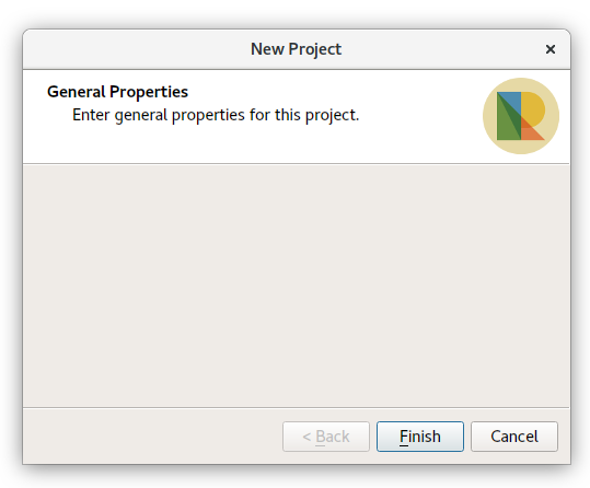
We’ll start super simple, creating a single page wizard with no settings. To do this we first create a Page1 subclass of QWizardPage, a ProjectWizard subclass of QWizard, and a simple runNewProjectWizard function which launches the wizard. (The code below is designed for QGIS 3.0, but will run with only small modifications on QGIS 2.x):


class Page1(QWizardPage):

    def __init__(self, parent=None):
        super().__init__(parent)
        self.setTitle('General Properties')
        self.setSubTitle('Enter general properties for this project.')


class ProjectWizard(QWizard):
    
    def __init__(self, parent=None):
        super().__init__(parent)
        
        self.addPage(Page1(self))
        self.setWindowTitle("New Project")


def runNewProjectWizard():
    d=ProjectWizard()
    d.exec()

If this code is executed in the QGIS Python console, you’ll see something like this:

Not too fancy (or functional) yet, but still not bad for 20 lines of code! We can instantly make this a bit nicer by inserting a custom logo into the widget. This is done by calling setPixmap inside the ProjectWizard constructor.


class ProjectWizard(QWizard):
    
    def __init__(self, parent=None):
        super().__init__(parent)
        
        self.addPage(Page1(self))
        self.setWindowTitle("New Project")

        logo_image = QImage('path_to_logo.png')
        self.setPixmap(QWizard.LogoPixmap, QPixmap.fromImage(logo_image))

That’s a bit nicer. QWizard has HEAPS of options for tweaking the wizards — best to read about those over at the Qt documentation. Our next step is to start adding some settings to this wizard. We’ll keep things easy for now and just insert a number of text input boxes (QLineEdits) into Page1:


class Page1(QWizardPage):

    def __init__(self, parent=None):
        super().__init__(parent)
        self.setTitle('General Properties')
        self.setSubTitle('Enter general properties for this project.')

        # create some widgets
        self.project_number_line_edit = QLineEdit()
        self.project_title_line_edit = QLineEdit()
        self.author_line_edit = QLineEdit()        
        
        # set the page layout
        layout = QGridLayout()
        layout.addWidget(QLabel('Project Number'),0,0)
        layout.addWidget(self.project_number_line_edit,0,1)
        layout.addWidget(QLabel('Title'),1,0)
        layout.addWidget(self.project_title_line_edit,1,1)
        layout.addWidget(QLabel('Author'),2,0)
        layout.addWidget(self.author_line_edit,2,1)
        self.setLayout(layout)

There’s nothing particularly new here, especially if you’ve used Qt widgets before. We make a number of QLineEdit widgets, and then create a grid layout containing these widgets and accompanying labels (QLabels). Here’s the result if we run our wizard now:

So now there’s the option to enter a project number, title and author. The next step is to force users to populate these fields before they can complete the wizard. Fortunately, QWizardPage has us covered here and we can use the registerField() function to do this. By calling registerField, we make the wizard aware of the settings we’ve added on this page, allowing us to retrieve their values when the wizard completes. We can also use registerField to automatically force their population by appending a * to the end of the field names. Just like this…

class Page1(QWizardPage):
    def __init__(self, parent=None):
        super().__init__(parent)
        ...
        self.registerField('number*',self.project_number_line_edit)
        self.registerField('title*',self.project_title_line_edit)
        self.registerField('author*',self.author_line_edit)

If we ran the wizard now, we’d be forced to enter something for project number, title and author before the Finish button becomes enabled. Neat! By registering the fields, we’ve also allowed their values to be retrieved after the wizard completes. Let’s alter runNewProjectWizard to retrieve these values and do something with them:

def runNewProjectWizard():
   d=ProjectWizard()
   d.exec()

   # Set the project title
   title=d.field('title')
   QgsProject.instance().setTitle(d.field('title'))

   # Create expression variables for the author and project number
   number=d.field('number')
   QgsExpressionContextUtils.setProjectVariable(QgsProject.instance(),'project_number', number)
   author=d.field('author')
   QgsExpressionContextUtils.setProjectVariable(QgsProject.instance(),'project_author', author)
 

Here, we set the project title directly and create expression variables for the project number and author. This allows their use within QGIS expressions via the @project_number and @project_author variables. Accordingly, they can be embedded into print layout templates so that layout elements are automatically populated with the corresponding author and project number. Nifty!

Ok, let’s beef up our wizard by adding a second page, asking the user to select a sensible projection (coordinate reference system) for their project. Thanks to improvements in QGIS 3.0, it’s super-easy to embed a powerful pre-made projection selector widget into your scripts, which even includes a handy preview of the area of the world that the projection is valid for.


class Page2(QWizardPage):

    def __init__(self, parent=None):
        super().__init__(parent)
        self.setTitle('Project Coordinate System')
        self.setSubTitle('Choosing an appropriate projection is important to ensure accurate distance and area measurements.')
        
        self.proj_selector = QgsProjectionSelectionTreeWidget()
        layout = QVBoxLayout()
        layout.addWidget(self.proj_selector)
        self.setLayout(layout)
        
        self.registerField('crs',self.proj_selector)
        self.proj_selector.crsSelected.connect(self.crs_selected)
        
    def crs_selected(self):
        self.setField('crs',self.proj_selector.crs())
        self.completeChanged.emit()
        
    def isComplete(self):
        return self.proj_selector.crs().isValid()

There’s a lot happening here. First, we subclass QWizardPage to create a second page in our widget. Then, just like before, we add some widgets to this page and set the page’s layout. In this case we are using the standard QgsProjectionSelectionTreeWidget to give users a projection choice. Again, we let the wizard know about our new setting by a call to registerField. However, since QWizard has no knowledge about how to handle a QgsProjectionSelectionTreeWidget, there’s a bit more to do here. So we make a connection to the projection selector’s crsSelected signal, hooking it up to a function which sets the wizard’s “crs” field value to the widget’s selected CRS. Here, we also emit the completeChanged signal, which indicates that the wizard page should re-validate the current settings. Lastly, we override QWizardPage’s isComplete method, checking that there’s a valid CRS selection in the selector widget. If we run the wizard now we’ll be forced to choose a valid CRS from the widget before the wizard allows us to proceed:

Lastly, we need to adapt runNewProjectWizard to also handle the projection setting:


def runNewProjectWizard():
    d=ProjectWizard()
    d.exec()

    # Set the project crs
    crs=d.field('crs')
    QgsProject.instance().setCrs(crs)

    # Set the project title
    title=d.field('title')
    ...

Great! A fully functional New Project wizard. The final piece of the puzzle is triggering this wizard when a user creates a new project within QGIS. To do this, we hook into the iface.newProjectCreated signal. By connecting to this signal, our code will be called whenever the user creates a new project (after all the logic for saving and closing the current project has been performed). It’s as simple as this:


iface.newProjectCreated.connect(runNewProjectWizard)

Now, whenever a new project is made, our wizard is triggered – forcing users to populate the required fields and setting up the project accordingly!

There’s one last little bit to do – we also need to prevent users cancelling or closing the wizard before completing it. That’s done by changing a couple of settings in the ProjectWizard constructor, and by overriding the default reject method (which prevents closing the dialog by pressing escape).


class ProjectWizard(QWizard):
    
    def __init__(self, parent=None):
        super().__init__(parent)
        ...
        self.setOption(QWizard.NoCancelButton, True)
        self.setWindowFlags(self.windowFlags() | QtCore.Qt.CustomizeWindowHint)
        self.setWindowFlags(self.windowFlags() & ~QtCore.Qt.WindowCloseButtonHint)

    def reject(self):
        pass

Here’s the full version of our code, ready for copying and pasting into the QGIS Python console:


icon_path = '/home/nyall/nr_logo.png'

class ProjectWizard(QWizard):
    
    def __init__(self, parent=None):
        super().__init__(parent)
        
        self.addPage(Page1(self))
        self.addPage(Page2(self))
        self.setWindowTitle("New Project")
        
        logo_image=QImage('path_to_logo.png')
        self.setPixmap(QWizard.LogoPixmap, QPixmap.fromImage(logo_image))
        
        self.setOption(QWizard.NoCancelButton, True)
        self.setWindowFlags(self.windowFlags() | QtCore.Qt.CustomizeWindowHint)
        self.setWindowFlags(self.windowFlags() & ~QtCore.Qt.WindowCloseButtonHint)
    def reject(self):
        pass
class Page1(QWizardPage):
    
    def __init__(self, parent=None):
        super().__init__(parent)
        self.setTitle('General Properties')
        self.setSubTitle('Enter general properties for this project.')

        # create some widgets
        self.project_number_line_edit = QLineEdit()
        self.project_title_line_edit = QLineEdit()
        self.author_line_edit = QLineEdit()        
        
        # set the page layout
        layout = QGridLayout()
        layout.addWidget(QLabel('Project Number'),0,0)
        layout.addWidget(self.project_number_line_edit,0,1)
        layout.addWidget(QLabel('Title'),1,0)
        layout.addWidget(self.project_title_line_edit,1,1)
        layout.addWidget(QLabel('Author'),2,0)
        layout.addWidget(self.author_line_edit,2,1)
        self.setLayout(layout)
        
        self.registerField('number*',self.project_number_line_edit)
        self.registerField('title*',self.project_title_line_edit)
        self.registerField('author*',self.author_line_edit)
 
 
class Page2(QWizardPage):
    
    def __init__(self, parent=None):
        super().__init__(parent)
        self.setTitle('Project Coordinate System')
        self.setSubTitle('Choosing an appropriate projection is important to ensure accurate distance and area measurements.')
        
        self.proj_selector = QgsProjectionSelectionTreeWidget()
        layout = QVBoxLayout()
        layout.addWidget(self.proj_selector)
        self.setLayout(layout)
        
        self.registerField('crs',self.proj_selector)
        self.proj_selector.crsSelected.connect(self.crs_selected)
        
    def crs_selected(self):
        self.setField('crs',self.proj_selector.crs())
        self.completeChanged.emit()
        
    def isComplete(self):
        return self.proj_selector.crs().isValid()
 
        
def runNewProjectWizard():
    d=ProjectWizard()
    d.exec()
    
    # Set the project crs
    crs=d.field('crs')
    QgsProject.instance().setCrs(crs)
    
    # Set the project title
    title=d.field('title')
    QgsProject.instance().setTitle(d.field('title'))

    # Create expression variables for the author and project number
    number=d.field('number')
    QgsExpressionContextUtils.setProjectVariable(QgsProject.instance(),'project_number', number)
    author=d.field('author')
    QgsExpressionContextUtils.setProjectVariable(QgsProject.instance(),'project_author', author)
    
    
iface.newProjectCreated.connect(runNewProjectWizard)

Quick Guide to Getting Started with PyQGIS 3 on Windows

Getting started with Python and QGIS 3 can be a bit overwhelming. In this post we give you a quick start to get you up and running and maybe make your PyQGIS life a little easier.

There are likely many ways to setup a working PyQGIS development environment---this one works pretty well.

Contents

Requirements

  • OSGeo4W Advanced Install of QGIS
  • pip (for installing/managing Python packages)
  • pb_tool (cross-platform tool for compiling/deploying/distributing QGIS plugin)
  • A customized startup script to set the environment (pyqgis.cmd)
  • IDE (optional)
  • Emacs (just kidding)
  • Vim (just kidding)

We'll start with the installs.

Installing

Almost everything we need can be installed using the OSGeo4W installer available on the QGIS website.

OSGeo4W

From the QGIS website, download the appropriate network installer (32 or 64 bit) for QGIS 3.

  • Run the installer and choose the Advanced Install option
  • Install from Internet
  • Choose a directory for the install---I prefer a path without spaces such as C:\OSGeo4W
  • Accept default for local package directory and Start menu name
  • Tweak network connection option if needed on the Select Your Internet Connection screen
  • Accept default download site location
  • From the Select packages screen, select: Desktop -> qgis: QGIS Desktop

When you click Next a bunch of additional packages will be suggested---just accept them and continue the install.

Once complete you will have a functioning QGIS install along with the other parts we need. If you want to work with the nightly build of QGIS, choose Desktop -> qgis-dev instead.

If you installed QGIS using the standalone installer, the easiest option is to remove it and install from OSGeo4W. You can run both the standalone and OSGeo4W versions on the same machine, but you need to be extra careful not to mix up the environment.

Setting the Environment

To continue with the setup, we need to set the environment by creating a .cmd script. The following is adapted from several sources, and trimmed down to the minimum. Copy and paste it into a file named pyqgis.cmd and save it to a convenient location (like your HOME directory).

@echo off
SET OSGEO4W_ROOT=C:\OSGeo4W3
call "%OSGEO4W_ROOT%"\bin\o4w_env.bat
call "%OSGEO4W_ROOT%"\apps\grass\grass-7.4.0\etc\env.bat
@echo off
path %PATH%;%OSGEO4W_ROOT%\apps\qgis-dev\bin
path %PATH%;%OSGEO4W_ROOT%\apps\grass\grass-7.4.0\lib
path %PATH%;C:\OSGeo4W3\apps\Qt5\bin
path %PATH%;C:\OSGeo4W3\apps\Python36\Scripts

set PYTHONPATH=%PYTHONPATH%;%OSGEO4W_ROOT%\apps\qgis-dev\python
set PYTHONHOME=%OSGEO4W_ROOT%\apps\Python36

set PATH=C:\Program Files\Git\bin;%PATH%

cmd.exe

You should customize the set PATH statement to add any paths you want available when working from the command line. I added paths to my git install.

The last line starts a cmd shell with the settings specified above it. We'll see an example of starting an IDE in a bit.

You can test to make sure all is well by double-clicking on our pyqgis.cmd script, then starting Python and attempting to import one of the QGIS modules:

C:\Users\gsherman>python3
Python 3.6.0 (v3.6.0:41df79263a11, Dec 23 2016, 07:18:10) [MSC v.1900 32 bit (In tel)] on win32
Type "help", "copyright", "credits" or "license" for more information.
>>> import qgis.core
>>> import PyQt5.QtCore

If you don't get any complaints on import, things are looking good.

Installing pb_tool

Open your customized shell (double-click on pyqgis.cmd to start it) to install pb_tool:

python3 -m pip install pb_tool

Check to see if pb_tool is installed correctly:

C:\Users\gsherman>pb_tool
Usage: pb_tool [OPTIONS] COMMAND [ARGS]...

  Simple Python tool to compile and deploy a QGIS plugin. For help on a
  command use --help after the command: pb_tool deploy --help.

  pb_tool requires a configuration file (default: pb_tool.cfg) that declares
  the files and resources used in your plugin. Plugin Builder 2.6.0 creates
  a config file when you generate a new plugin template.

  See http://g-sherman.github.io/plugin_build_tool for for an example config
  file. You can also use the create command to generate a best-guess config
  file for an existing project, then tweak as needed.

  Bugs and enhancement requests, see:
  https://github.com/g-sherman/plugin_build_tool

Options:
  --help  Show this message and exit.

Commands:
  clean       Remove compiled resource and ui files
  clean_docs  Remove the built HTML help files from the...
  compile     Compile the resource and ui files
  config      Create a config file based on source files in...
  create      Create a new plugin in the current directory...
  dclean      Remove the deployed plugin from the...
  deploy      Deploy the plugin to QGIS plugin directory...
  doc         Build HTML version of the help files using...
  help        Open the pb_tools web page in your default...
  list        List the contents of the configuration file
  translate   Build translations using lrelease.
  update      Check for update to pb_tool
  validate    Check the pb_tool.cfg file for mandatory...
  version     Return the version of pb_tool and exit
  zip         Package the plugin into a zip file suitable...

If you get an error, make sure C:\OSGeo4W3\apps\Python36\Scripts is in your PATH.

More information on using pb_tool is available on the project website.

Working on the Command Line

Just double-click on your pyqgis.cmd script from the Explorer or a desktop shortcut to start a cmd shell. From here you can use Python interactively and also use pb_tool to compile and deploy your plugin for testing.

IDE Example

By adding one line to our pyqgis.cmd script, we can start our IDE with the proper settings to recognize the QGIS libraries:

start "PyCharm aware of Quantum GIS" /B "C:\Program Files (x86)\JetBrains\PyCharm 3.4.1\bin\pycharm.exe" %*

We added the start statement with the path to the IDE (in this case PyCharm). If you save this to something like pycharm.cmd, you can double-click on it to start PyCharm. The same method works for other IDEs, such as PyDev.

Within your IDE settings, point it to use the Python interpreter included with OSGeo4W---typically at: %OSGEO4W_ROOT%\bin\python3.exe. This will make it pick up all the QGIS goodies needed for development, completion, and debugging. In my case OSGEO4W_ROOT is C:\OSGeo4W3, so in the IDE, the path to the correct Python interpreter would be: C:\OSGeo4W3\bin\python3.exe.

Make sure you adjust the paths in your .cmd scripts to match your system and software locations.

Workflow

Here is an example of a workflow you can use once you're setup for development.

Creating a New Plugin

  1. Use the Plugin Builder plugin to create a starting point [1]
  2. Start your pyqgis.cmd shell
  3. Use pb_tool to compile and deploy the plugin (pb_tool deploy will do it all in one pass)
  4. Activate it in QGIS and test it out
  5. Add code, deploy, test, repeat

Working with Existing Plugin Code

The steps are basically the same was creating a new plugin, except we start by using pb_tool to create a new config file:

  1. Start your pyqgis.cmd shell
  2. Change to the directory containing your plugin code
  3. Use pb_tool create to create a config file
  4. Edit pb_tool.cfg to adjust/add things create may have missed
  5. Start at step 3 in Creating a New Plugin and press on

Troubleshooting

Assuming you have things properly installed, trouble usually stems from an incorrect environment.

  • Make sure QGIS runs and the Python console is available and working
  • Check all the paths in your pygis.cmd or your custom IDE cmd script
  • Make sure your IDE is using the Python interpreter that comes with OSGeo4W


[1] Plugin Builder 3.x generates a pb_tool config file

OSM data quality assessment: producing map to illustrate data quality

At Oslandia, we like working with Open Source tool projects and handling Open (geospatial) Data. In this article series, we will play with the OpenStreetMap (OSM) map and subsequent data. Here comes the eighth article of this series, dedicated to the OSM data quality evaluation, through production of new maps.

1 Description of OSM element

 1.1 Element metadata extraction

As mentionned in a previous article dedicated to metadata extraction, we have to focus on element metadata itself if we want to produce valuable information about quality. The first questions to answer here are straightforward: what is an OSM element? and how to extract its associated metadata?. This part is relatively similar to the job already done with users.

We know from previous analysis that an element is created during a changeset by a given contributor, may be modified several times by whoever, and may be deleted as well. This kind of object may be either a “node”, a “way” or a “relation”. We also know that there may be a set of different tags associated with the element. Of course the list of every operations associated to each element is recorded in the OSM data history. Let’s consider data around Bordeaux, as in previous blog posts:

import pandas as pd
elements = pd.read_table('../src/data/output-extracts/bordeaux-metropole/bordeaux-metropole-elements.csv', parse_dates=['ts'], index_col=0, sep=",")
elements.head().T
   elem        id  version  visible         ts    uid  chgset
0  node  21457126        2    False 2008-01-17  24281  653744
1  node  21457126        3    False 2008-01-17  24281  653744
2  node  21457126        4    False 2008-01-17  24281  653744
3  node  21457126        5    False 2008-01-17  24281  653744
4  node  21457126        6    False 2008-01-17  24281  653744

This short description helps us to identify some basic features, which are built in the following snippets. First we recover the temporal features:

elem_md = (elements.groupby(['elem', 'id'])['ts']
            .agg(["min", "max"])
            .reset_index())
elem_md.columns = ['elem', 'id', 'first_at', 'last_at']
elem_md['lifespan'] = (elem_md.last_at - elem_md.first_at)/pd.Timedelta('1D')
extraction_date = elements.ts.max()
elem_md['n_days_since_creation'] = ((extraction_date - elem_md.first_at)
                                  / pd.Timedelta('1d'))
elem_md['n_days_of_activity'] = (elements
                              .groupby(['elem', 'id'])['ts']
                              .nunique()
                              .reset_index())['ts']
elem_md = elem_md.sort_values(by=['first_at'])
                                    213418
elem                                  node
id                               922827508
first_at               2010-09-23 00:00:00
last_at                2010-09-23 00:00:00
lifespan                                 0
n_days_since_creation                 2341
n_days_of_activity                       1

Then the remainder of the variables, e.g. how many versions, contributors, changesets per elements:

    elem_md['version'] = (elements.groupby(['elem','id'])['version']
                          .max()
                          .reset_index())['version']
    elem_md['n_chgset'] = (elements.groupby(['elem', 'id'])['chgset']
                           .nunique()
                           .reset_index())['chgset']
    elem_md['n_user'] = (elements.groupby(['elem', 'id'])['uid']
                         .nunique()
                         .reset_index())['uid']
    osmelem_last_user = (elements
                         .groupby(['elem','id'])['uid']
                         .last()
                         .reset_index())
    osmelem_last_user = osmelem_last_user.rename(columns={'uid':'last_uid'})
    elements = pd.merge(elements, osmelem_last_user,
                       on=['elem', 'id'])
    elem_md = pd.merge(elem_md,
                       elements[['elem', 'id', 'version', 'visible', 'last_uid']],
                       on=['elem', 'id', 'version'])
    elem_md = elem_md.set_index(['elem', 'id'])
    elem_md.sample().T
elem                                  node
id                              1340445266
first_at               2011-06-26 00:00:00
last_at                2011-06-27 00:00:00
lifespan                                 1
n_days_since_creation                 2065
n_days_of_activity                       2
version                                  2
n_chgset                                 2
n_user                                   1
visible                              False
last_uid                            354363

As an illustration we have above an old two-versionned node, no more visible on the OSM website.

1.2 Characterize OSM elements with user classification

This set of features is only descriptive, we have to add more information to be able to characterize OSM data quality. That is the moment to exploit the user classification produced in the last blog post!

As a recall, we hypothesized that clustering the users permits to evaluate their trustworthiness as OSM contributors. They are either beginners, or intermediate users, or even OSM experts, according to previous classification.

Each OSM entity may have received one or more contributions by users of each group. Let’s say the entity quality is good if its last contributor is experienced. That leads us to classify the OSM entities themselves in return!

How to include this information into element metadata?

We first need to recover the results of our clustering process.

user_groups = pd.read_hdf("../src/data/output-extracts/bordeaux-metropole/bordeaux-metropole-user-kmeans.h5", "/individuals")
user_groups.head()
           PC1       PC2       PC3       PC4       PC5       PC6  Xclust
uid                                                                     
1626 -0.035154  1.607427  0.399929 -0.808851 -0.152308 -0.753506       2
1399 -0.295486 -0.743364  0.149797 -1.252119  0.128276 -0.292328       0
2488  0.003268  1.073443  0.738236 -0.534716 -0.489454 -0.333533       2
5657 -0.889706  0.986024  0.442302 -1.046582 -0.118883 -0.408223       4
3980 -0.115455 -0.373598  0.906908  0.252670  0.207824 -0.575960       5

As a remark, there were several important results to save after the clustering process; we decided to serialize them into a single binary file. Pandas knows how to manage such file, that would be a pity not to take advantage of it!

We recover the individuals groups in the eponym binary file tab (column Xclust), and only have to join it to element metadata as follows:

elem_md = elem_md.join(user_groups.Xclust, on='last_uid')
elem_md = elem_md.rename(columns={'Xclust':'last_uid_group'})
elem_md.reset_index().to_csv("../src/data/output-extracts/bordeaux-metropole/bordeaux-metropole-element-metadata.csv")
elem_md.sample().T
elem                                  node
id                              1530907753
first_at               2011-12-04 00:00:00
last_at                2011-12-04 00:00:00
lifespan                                 0
n_days_since_creation                 1904
n_days_of_activity                       1
version                                  1
n_chgset                                 1
n_user                                   1
visible                               True
last_uid                             37548
last_uid_group                           2

From now, we can use the last contributor cluster as an additional information to generate maps, so as to study data quality…

Wait… There miss another information, isn’t it? Well yes, maybe the most important one, when dealing with geospatial data: the location itself!

1.3 Recover the geometry information

Even if Pyosmium library is able to retrieve OSM element geometries, we realized some tests with an other OSM data parser here: osm2pgsql.

We can recover geometries from standard OSM data with this tool, by assuming the existence of an osm database, owned by user:

osm2pgsql -E 27572 -d osm -U user -p bordeaux_metropole --hstore ../src/data/raw/bordeaux-metropole.osm.pbf

We specify a France-focused SRID (27572), and a prefix for naming output databases point, line, polygon and roads.

We can work with the line subset, that contains the physical roads, among other structures (it roughly corresponds to the OSM ways), and build an enriched version of element metadata, with geometries.

First we can create the table bordeaux_metropole_geomelements, that will contain our metadata…

DROP TABLE IF EXISTS bordeaux_metropole_elements;
DROP TABLE IF EXISTS bordeaux_metropole_geomelements;
CREATE TABLE bordeaux_metropole_elements(
       id int,
       elem varchar,
       osm_id bigint,
       first_at varchar,
       last_at varchar,
       lifespan float,
       n_days_since_creation float,
       n_days_of_activity float,
       version int,
       n_chgsets int,
       n_users int,
       visible boolean,
       last_uid int,
       last_user_group int
);

…then, populate it with the data accurate .csv file…

COPY bordeaux_metropole_elements
FROM '/home/rde/data/osm-history/output-extracts/bordeaux-metropole/bordeaux-metropole-element-metadata.csv'
WITH(FORMAT CSV, HEADER, QUOTE '"');

…and finally, merge the metadata with the data gathered with osm2pgsql, that contains geometries.

SELECT l.osm_id, h.lifespan, h.n_days_since_creation,
h.version, h.visible, h.n_users, h.n_chgsets,
h.last_user_group, l.way AS geom
INTO bordeaux_metropole_geomelements
FROM bordeaux_metropole_elements as h
INNER JOIN bordeaux_metropole_line as l
ON h.osm_id = l.osm_id AND h.version = l.osm_version
WHERE l.highway IS NOT NULL AND h.elem = 'way'
ORDER BY l.osm_id;

Wow, this is wonderful, we have everything we need in order to produce new maps, so let’s do it!

2 Keep it visual, man!

From the last developments and some hypothesis about element quality, we are able to produce some customized maps. If each OSM entities (e.g. roads) can be characterized, then we can draw quality maps by highlighting the most trustworthy entities, as well as those with which we have to stay cautious.

In this post we will continue to focus on roads within the Bordeaux area. The different maps will be produced with the help of Qgis.

2.1 First step: simple metadata plotting

As a first insight on OSM elements, we can plot each OSM ways regarding simple features like the number of users who have contributed, the number of version or the element anteriority.

Figure 1: Number of active contributors per OSM way in Bordeaux


Figure 2: Number of versions per OSM way in Bordeaux

With the first two maps, we see that the ring around Bordeaux is the most intensively modified part of the road network: more unique contributors are implied in the way completion, and more versions are designed for each element. Some major roads within the city center present the same characteristics.

Figure 3: Anteriority of each OSM way in Bordeaux, in years

If we consider the anteriority of OSM roads, we have a different but interesting insight of the area. The oldest roads are mainly located within the city center, even if there are some exceptions. It is also interesting to notice that some spatial patterns arise with temporality: entire neighborhoods are mapped within the same anteriority.

2.2 More complex: OSM data merging with alternative geospatial representations

To go deeper into the mapping analysis, we can use the INSEE carroyed data, that divides France into 200-meter squared tiles. As a corollary OSM element statistics may be aggregated into each tile, to produce additional maps. Unfortunately an information loss will occur, as such tiles are only defined where people lives. However it can provides an interesting alternative illustration.

To exploit such new data set, we have to merge the previous table with the accurate INSEE table. Creating indexes on them is of great interest before running such a merging operation:

CREATE INDEX insee_geom_gist
ON open_data.insee_200_carreau USING GIST(wkb_geometry);
CREATE INDEX osm_geom_gist
ON bordeaux_metropole_geomelements USING GIST(geom);

DROP TABLE IF EXISTS bordeaux_metropole_carroyed_ways;
CREATE TABLE bordeaux_metropole_carroyed_ways AS (
SELECT insee.ogc_fid, count(*) AS nb_ways,
avg(bm.version) AS avg_version, avg(bm.lifespan) AS avg_lifespan,
avg(bm.n_days_since_creation) AS avg_anteriority,
avg(bm.n_users) AS avg_n_users, avg(bm.n_chgsets) AS avg_n_chgsets,
insee.wkb_geometry AS geom
FROM open_data.insee_200_carreau AS insee
JOIN bordeaux_metropole_geomelements AS bm
ON ST_Intersects(insee.wkb_geometry, bm.geom)
GROUP BY insee.ogc_fid
);

As a consequence, we get only 5468 individuals (tiles), a quantity that must be compared to the 29427 roads previously handled… This operation will also simplify the map analysis!

We can propose another version of previous maps by using Qgis, let’s consider the average number of contributors per OSM roads, for each tile:

Figure 4: Number of contributors per OSM roads, aggregated by INSEE tile

2.3 The cherry on the cake: representation of OSM elements with respect to quality

Last but not least, the information about last user cluster can shed some light on OSM data quality: by plotting each roads according to the last user who has contributed, we might identify questionable OSM elements!

We simply have to design similar map than in previous section, with user classification information:

Figure 5: OSM roads around Bordeaux, according to the last user cluster (1: C1, relation experts; 2: C0, versatile expert contributors; 3: C4, recent one-shot way contributors; 4: C3, old one-shot way contributors; 5: C5, locally-unexperienced way specialists)

According to the clustering done in the previous article (be careful, the legend is not the same here…), we can make some additional hypothesis:

  • Light-blue roads are OK, they correspond to the most trustful cluster of contributors (91.4% of roads in this example)
  • There is no group-0 road (group 0 corresponds to cluster C2 in the previous article)… And that’s comforting! It seems that “untrustworthy” users do not contribute to roads or -more probably- that their contributions are quickly amended.
  • Other contributions are made by intermediate users: a finer analysis should be undertaken to decide if the corresponding elements are valid. For now, we can consider everything is OK, even if local patterns seem strong. Areas of interest should be verified (they are not necessarily of low quality!)

For sure, it gives a fairly new picture of OSM data quality!

3 Conclusion

In this last article, we have designed new maps on a small area, starting from element metadata. You have seen the conclusion of our analysis: characterizing the OSM data quality starting from the user contribution history.

Of course some works still have to be done, however we detailed a whole methodology to tackle the problem. We hope you will be able to reproduce it, and to design your own maps!

Feel free to contact us if you are interested in this topic!

Speeding up your PyQGIS scripts

I’ve recently spent some time optimising the performance of various QGIS plugins and algorithms, and I’ve noticed that there’s a few common performance traps which developers fall into when fetching features from a vector layer. In this post I’m going to explore these traps, what makes them slow, and how to avoid them.

As a bit of background, features are fetched from a vector layer in QGIS using a QgsFeatureRequest object. Common use is something like this:

request = QgsFeatureRequest()
for feature in vector_layer.getFeatures(request):
    # do something

This code would iterate over all the features in layer. Filtering the features is done by tweaking the QgsFeatureRequest, such as:

request = QgsFeatureRequest().setFilterFid(1001)
feature_1001 = next(vector_layer.getFeatures(request))

In this case calling getFeatures(request) just returns the single feature with an ID of 1001 (which is why we shortcut and use next(…) here instead of iterating over the results).

Now, here’s the trap: calling getFeatures is expensive. If you call it on a vector layer, QGIS will be required to setup an new connection to the data store (the layer provider), create some query to return data, and parse each result as it is returned from the provider. This can be slow, especially if you’re working with some type of remote layer, such as a PostGIS table over a VPN connection. This brings us to our first trap:

Trap #1: Minimise the calls to getFeatures()

A common task in PyQGIS code is to take a list of feature IDs and then request those features from the layer. A see a lot of older code which does this using something like:

for id in some_list_of_feature_ids:
    request = QgsFeatureRequest().setFilterFid(id)
    feature = next(vector_layer.getFeatures(request))
    # do something with the feature

Why is this a bad idea? Well, remember that every time you call getFeatures() QGIS needs to do a whole bunch of things before it can start giving you the matching features. In this case, the code is calling getFeatures() once for every feature ID in the list. So if the list had 100 features, that means QGIS is having to create a connection to the data source, set up and prepare a query to match a single feature, wait for the provider to process that, and then finally parse the single feature result. That’s a lot of wasted processing!

If the code is rewritten to take the call to getFeatures() outside of the loop, then the result is:

request = QgsFeatureRequest().setFilterFids(some_list_of_feature_ids)
for feature in vector_layer.getFeatures(request):
    # do something with the feature

Now there’s just a single call to getFeatures() here. QGIS optimises this request by using a single connection to the data source, preparing the query just once, and fetching the results in appropriately sized batches. The difference is huge, especially if you’re dealing with a large number of features.

Trap #2: Use QgsFeatureRequest filters appropriately

Here’s another common mistake I see in PyQGIS code. I often see this one when an author is trying to do something with all the selected features in a layer:

for feature in vector_layer.getFeatures():
    if not feature.id() in vector_layer.selectedFeaturesIds():
        continue

    # do something with the feature

What’s happening here is that the code is iterating over all the features in the layer, and then skipping over any which aren’t in the list of selected features. See the problem here? This code iterates over EVERY feature in the layer. If you’re layer has 10 million features, we are fetching every one of these from the data source, going through all the work of parsing it into a QGIS feature, and then promptly discarding it if it’s not in our list of selected features. It’s very inefficient, especially if fetching features is slow (such as when connecting to a remote database source).

Instead, this code should use the setFilterFids() method for QgsFeatureRequest:

request = QgsFeatureRequest().setFilterFids(vector_layer.selectedFeaturesIds())
for feature in vector_layer.getFeatures(request):
    # do something with the feature

Now, QGIS will only fetch features from the provider with matching feature IDs from the list. Instead of fetching and processing every feature in the layer, only the actual selected features will be fetched. It’s not uncommon to see operations which previously took many minutes (or hours!) drop down to a few seconds after applying this fix.

Another variant of this trap uses expressions to test the returned features:

filter_expression = QgsExpression('my_field &gt; 20')
for feature in vector_layer.getFeatures():
    if not filter_expression.evaluate(feature):
        continue

    # do something with the feature

Again, this code is fetching every single feature from the layer and then discarding it if it doesn’t match the “my_field > 20” filter expression. By rewriting this to:

request = QgsFeatureRequest().setFilterExpression('my_field &gt; 20')
for feature in vector_layer.getFeatures(request):
    # do something with the feature

we hand over the bulk of the filtering to the data source itself. Recent QGIS versions intelligently translate the filter into a format which can be applied directly at the provider, meaning that any relevant indexes and other optimisations can be applied by the provider itself. In this case the rewritten code means that ONLY the features matching the ‘my_field > 20’ criteria are fetched from the provider – there’s no time wasted messing around with features we don’t need.


Trap #3: Only request values you need

The last trap I often see is that more values are requested from the layer then are actually required. Let’s take the code:

my_sum = 0
for feature in vector_layer.getFeatures(request):
    my_sum += feature['value']

In this case there’s no way we can optimise the filters applied, since we need to process every feature in the layer. But – this code is still inefficient. By default QGIS will fetch all the details for a feature from the provider. This includes all attribute values and the feature’s geometry. That’s a lot of processing – QGIS needs to transform the values from their original format into a format usable by QGIS, and the feature’s geometry needs to be parsed from it’s original type and rebuilt as a QgsGeometry object. In our sample code above we aren’t doing anything with the geometry, and we are only using a single attribute from the layer. By calling setFlags( QgsFeatureRequest.NoGeometry ) and setSubsetOfAttributes() we can tell QGIS that we don’t need the geometry, and we only require a single attribute’s value:

my_sum = 0
request = QgsFeatureRequest().setFlags(QgsFeatureRequest.NoGeometry).setSubsetOfAttributes(['value'], vector_layer.fields() )
for feature in vector_layer.getFeatures(request):
    my_sum += feature['value']

None of the unnecessary geometry parsing will occur, and only the ‘value’ attribute will be fetched and populated in the features. This cuts down both on the processing required AND the amount of data transfer between the layer’s provider and QGIS. It’s a significant improvement if you’re dealing with larger layers.

Conclusion

Optimising your feature requests is one of the easiest ways to speed up your PyQGIS script! It’s worth spending some time looking over all your uses of getFeatures() to see whether you can cut down on what you’re requesting – the results can often be mind blowing!

The road to QGIS 3.0 – part 1

qgis_icon.svgAs we discussed in QGIS 3 is under way, the QGIS project is working toward the next major version of the application and these developments have major impact on any custom scripts or plugins you’ve developed for QGIS.

We’re now just over a week into this work, and already there’s been tons of API breaking changes landing the code base. In this post we’ll explore some of these changes, what’s motivated them, and what they mean for your scripts.

The best source for keeping track of these breaking changes is to watch the API break documentation on GitHub. This file is updated whenever a change lands which potentially breaks plugins/scripts, and will eventually become a low-level guide to porting plugins to QGIS 3.0.

API clean-ups

So far, lots of the changes which have landed have related to cleaning up the existing API. These include:

Removal of deprecated API calls

The API has been frozen since QGIS 2.0 was released in 2013, and in the years since then many things have changed. As a result, different parts of the API were deprecated along the way as newer, better ways of doing things were introduced. The deprecated code was left intact so that QGIS 2.x plugins would still all function correctly. By removing these older, deprecated code paths it enables the QGIS developers to streamline the code, remove hacky workarounds, untested methods, and just generally “clean things up”. As an example, the older labelling system which pre-dates QGIS 2.0 (it had no collision detection, no curved labels, no fancy data defined properties or rule based labelling!) was still floating around just in case someone tried to open a QGIS 1.8 project. That’s all gone now, culling over 5000 lines of outdated, unmaintained code. Chances are this won’t affect your plugins in the slightest. Other removals, like the removal of QgsMapRenderer (the renderer used before multi-threaded rendering was introduced) likely have a much larger impact, as many scripts and plugins were still using QgsMapRenderer classes and calls. These all need to be migrated to the new QgsMapRendererJob and QgsMapSettings classes.

Renaming things for consistency

Consistent naming helps keep the API predictable and more user friendly. Lots of changes have landed so far to make the naming of classes and methods more consistent. These include things like:

  • Making sure names use consistent capitalization. Eg, there was previously methods named “writeXML” and “writeXml”. These have all been renamed to consistently use camel case, including for acronyms. (In case you’re wondering – this convention is used to follow the Qt library conventions).
  • Consistent use of terms. The API previously used a mix of “CRS” and “SRS” for similar purposes – it now consistently uses “CRS” for a coordinate reference system.
  • Removal of abbreviations. Lots of abbreviated words have been removed from the names, eg “destCrs” has become “destinationCrs”. The API wasn’t consistently using the same abbreviations (ie “dest”/”dst”/”destination”), so it was decided to remove all use of abbreviated words and replace them with the full word. This helps keep things predictable, and is also a bit friendlier for non-native English speakers.

The naming changes all need to be addressed to make existing scripts and plugins compatible with QGIS 3.0. It’s potentially quite a lot of work for plugin developers, but in the long term it will make the API easier to use.

Changes to return and argument types

There’s also been lots of changes relating to the types of objects returned by functions, or the types of objects used as function arguments. Most of these involve changing the c++ types from pointers to references, or from references to copies. These changes are being made to strengthen the API and avoid potential crashes. In most cases they don’t have any affect on PyQGIS code, with some exceptions:

  • Don’t pass Python “None” objects as QgsCoordinateReferenceSystems or as QgsCoordinateTransforms. In QGIS 3.0 you must pass invalid QgsCoordinateReferenceSystem objects (“QgsCoordinateReferenceSystem()”) or invalid QgsCoordinateTransform (“QgsCoordinateTransform()”) objects instead.

Transparent caching of CRS creation

The existing QgsCRSCache class has been removed. This class was used to cache the expensive results of initializing a QgsCoordinateReferenceSystem object, so that creating the same CRS could be done instantly and avoid slow databases lookups. In QGIS 3.0 this caching is now handled transparently, so there is no longer a need for the separate QgsCRSCache and it has been removed. If you were using QgsCRSCache in your PyQGIS code, it will need to be removed and replaced with the standard QgsCoordinateReferenceSystem constructors.

This change has the benefit that many existing plugins which were not explicitly using QgsCRSCache will now gain the benefits of the faster caching mechanism – potentially this could dramatically speed up existing plugin algorithms.

In summary

The QGIS developers have been busy fixing, improving and cleaning up the PyQGIS API. We recognise that these changes result in significant work for plugin and script developers, so we’re committed to providing quality documentation for how to adapt your code for these changes, and we will also investigate the use of automated tools to help ease your code transition to QGIS 3.0. We aren’t making changes lightly, but instead are carefully refining the API to make it more predictable, streamlined and stable.

If you’d like assistance with (or to outsource) the transition of your existing QGIS scripts and plugins to QGIS 3.0, just contact us at North Road to discuss. Every day we’re directly involved in the changes moving to QGIS 3.0, so we’re ideally placed to make this transition painless for you!

QGIS 3 is underway – what does it mean for your plugins and scripts?

With the imminent release of QGIS 2.16, the development attention has now shifted to the next scheduled release – QGIS 3.0! If you haven’t been following the discussion surrounding this I’m going to try and summarise what exactly 3.0 means and how it will impact any scripts or plugins you’ve developed for QGIS.

qgis_icon.svgQGIS 3.0 is the first major QGIS release since 2.0 was released way back in September 2013. Since that release so much has changed in QGIS… a quick glance over the release notes for 2.14 shows that even for this single point release there’s been hundreds of changes. Despite this, for all 2.x releases the PyQGIS API has remained stable, and a plugin or script which was developed for use in QGIS 2.0 will still work in QGIS 2.16.

Version 3.0 will introduce the first PyQGIS API break since 2013. An API break like this is required to move QGIS to newer libraries such as Qt 5 and Python 3, and allows the development team the flexibility to tackle long-standing issues and limitations which cannot be fixed using the 2.x API. Unfortunately, the side effect of this API break is that the scripts and plugins which you use in QGIS 2.x will no longer work when QGIS 3.0 is released!

Numerous API breaking changes have already started to flow into QGIS, and 2.16 isn’t even yet publicly available. The best way to track these changes is to keep an eye on the “API changes” documentation.  This document describes all the changes which are flowing in which affect PyQGIS code, and describe how best they should be addressed by plugin and script maintainers. Some changes are quite trivial and easy to update code for, others are more extreme (such as changes surrounding moving to PyQt5 and Python 3) and may require significant time to adapt for.

I’d encourage all plugin and script developers to keep watching the API break documentation, and subscribe to the developers list for additional information about required changes as they are introduced.

If you’re looking for assistance or to outsource adaptation of your plugins and scripts to QGIS 3.0 – the team at North Road are ideally placed to assist! Our team includes some of the most experienced QGIS developers who are directly involved with the development of QGIS 3.0, so you can be confident knowing that your code is in good hands. Just contact us to discuss your QGIS development requirements.

You can read more about QGIS 3.0 API changes in The road to QGIS 3.0 – part 1.

A new QGIS plugin allows dynamic filtering of values in forms


This plugin has been partially funded (50%) by ARPA Piemonte.

Description

This is a core-enhancement QGIS plugin that makes the implementation of complex dynamic filters in QGIS attribute forms an easy task. For example, this widget can be used to implement drill-down forms, where the values available in one field depend on the values of other fields.

Download

The plugin is available on the official QGIS Python Plugin Repository and the source code is on GitHub QGIS Form Value Relation plugin repository

Implementation

The new “Form Value Relation” widget is essentially a clone of the core “Value Relation” widget with some important differences: When the widget is created:
  • the whole unfiltered features of the related layer are loaded and cached
  • the form values of all the attributes are added to the context (see below)
  • the filtering against the expression happens every time the widget is refreshed
  • a signal is bound to the form changes and if the changed field is present in the filter expression, the features are filtered against the expression and the widget is refreshed

Using form values in the expression

A new expression function is available (in the “Custom” section):
CurrentFormValue('FIELD_NAME')
This function returns the current value of a field in the editor form.

Note

  1. This function can only be used inside forms and it’s particularly useful when used together with the custom widget `Form Value Relation`
  2. If the field does not exists the function returns an empty string.

Visual guide

  Download the example project.   This is the new widget in action: changing the field FK_PROV, the ISTAT values are filtered according to the filter expression.
The new widget in action

The new widget drill-down in action

layer_config_fields

Choosing the new widget

Configuring the widget

Configuring the widget

Configuring the expression

Configuring the expression to read FK_PROV value from the form

QGIS developer meeting in Nødebo

During the hackfest I’ve been working on the refactoring of the server component, aimed to wrap the server into a class and create python bindings for the new classes. This work is now in the PR queue and brings a first working python test for the server itself.

The server can now be invoked directly from python, like in the example below:


#!/usr/bin/env python
"""
Super simple QgsServer.
"""

from qgis.server import *
from BaseHTTPServer import *

class handler (BaseHTTPRequestHandler):

    server = QgsServer()

    def _doHeaders(self, response):
        l = response.pop(0)
        while l:
            h = l.split(':')
            self.send_header(h[0], ':'.join(h[1:]))
            self.log_message( "send_header %s - %s" % (h[0], ':'.join(h[1:])))
            l = response.pop(0)
        self.end_headers()

    def do_HEAD(self):
        self.send_response(200)
        response = str(handler.server.handleRequestGetHeaders(self.path[2:])).split('\n')
        self._doHeaders(response)

    def do_GET(self):
        response = str(handler.server.handleRequest(self.path[2:])).split('\n')
        i = 0
        self.send_response(200)
        self._doHeaders(response)
        self.wfile.write(('\n'.join(response[i:])).strip())

    def do_OPTIONS(s):
        handler.do_GET(s)

httpd = HTTPServer( ('', 8000), handler)

while True:
    httpd.handle_request()

The python bindings capture the server output instead of printing it on FCGI stdout and allow to pass the request parameters QUERY_STRING directly to the request handler as a string, this makes writing python tests very easy.

How to read a raster cell with Python QGIS and GDAL

QGIS and GDAL both have Python bindings, you can use both libraries to read a value from a raster cell, since QGIS uses GDAL libraries under the hood, we can expect to read the exact same value with both systems.


Here is a short example about how to do it with the two different approaches, we assume that you are working inside the QGIS python console and the project has a raster file loaded, but with just a few modifications, the example can also be run from a standard python console.

The example raster layer is a DTM with 1000 cells width and 2000 cells height, we want to read the value at the cell with coordinates x = 500 and y = 1000.

# First layer in QGIS project is a DTM 2 bands raster
from osgeo import gdal
# You need this to convert raw values readings from GDAL
import struct

# Read the cell with this raster coordinates
x = 500
y = 1000

# Get the map layer registry
reg = QgsMapLayerRegistry.instance()

# Get the first layer (the DTM raster)
qgis_layer = reg.mapLayers().values()[0]

# Open the raster with GDAL
gdal_layer = gdal.Open(rlayer.source())

"""
Fetches the coefficients for transforming between pixel/line (P,L) raster space, 
and projection coordinates (Xp,Yp) space.
    Xp = padfTransform[0] + P*padfTransform[1] + L*padfTransform[2];
    Yp = padfTransform[3] + P*padfTransform[4] + L*padfTransform[5];
In a north up image, padfTransform[1] is the pixel width, and padfTransform[5] 
is the pixel height. The upper left corner of the upper left pixel is 
at position (padfTransform[0],padfTransform[3]).
"""
gt = gldal_layer.GetGeoTransform()

# o:origin, r:rotation, s:size
xo, xs, xr, yo, yr, ys = gt

# Read band 1 at the middle of the raster ( x = 500, y = 1000)
band = gdal_layer.GetRasterBand(1)
gdal_value = struct.unpack('f', band.ReadRaster(x, y, 1, 1, buf_type=band.DataType))[0]

xcoo = xo + xs * x + xr * y
ycoo = yo + yr * x + ys * y

# Read the value with QGIS, we must pass the map coordinates
# and the exact extent = 1 cell size
qgis_value = qgis_layer.dataProvider().identify(QgsPoint(xcoo, ycoo), \
    QgsRaster.IdentifyFormatValue, \
    theExtent=QgsRectangle( xcoo , ycoo, xcoo + xs, ycoo + ys) )\
    .results()[1]

assert(gdal_value == qgis_value)

  • <<
  • Page 3 of 5 ( 95 posts )
  • >>
  • python

Back to Top

Sustaining Members