Related Plugins and Tags

QGIS Planet

Analyzing and visualizing large-scale fire events using QGIS processing with ST-DBSCAN

A while back, one of our ninjas added a new algorithm in QGIS’ processing toolbox named ST-DBSCAN Clustering, short for spatio temporal density-based spatial clustering of applications with noise. The algorithm regroups features falling within a user-defined maximum distance and time duration values.

This post will walk you through one practical use for the algorithm: large-scale fire event analysis and visualization through remote-sensed fire detection. More specifically, we will be looking into one of the larger fire events which occurred in Canada’s Quebec province in June 2023.

Fetching and preparing FIRMS data

NASA’s Fire Information for Resource Management System (FIRMS) offers a fantastic worldwide archive of all fire detected through three spaceborne sources: MODIS C6.1 with a resolution of roughly 1 kilometer as well as VIIRS S-NPP and VIIRS NOAA-20 with a resolution of 375 meters. Each detected fire is represented by a point that sits at the center of the source’s resolution grid.

Each source will cover the whole world several times per day. Since detection is impacted by atmospheric conditions, a given pass by one source might not be able to register an ongoing fire event. It’s therefore advisable to rely on more than one source.

To look into our fire event, we have chosen the two fire detection sources with higher resolution – VIIRS S-NPP and VIIRS NOAA-20 – covering the whole month of June 2023. The datasets were downloaded from FIRMS’ archive download page.

After downloading the two separate datasets, we combined them into one merged geopackage dataset using QGIS processing toolbox’s Merge Vector Layers algorithm. The merged dataset will be used to conduct the clustering analysis.

In addition, we will use QGIS’s field calculator to create a new Date & Time field named ACQ_DATE_TIME using the following expression:

to_datetime("ACQ_DATE" || "ACQ_TIME", 'yyyy-MM-ddhhmm')

This will allow us to calculate precise time differences between two dates.

Modeling and running the analysis

The large-scale fire event analysis requires running two distinct algorithms:

  • a spatiotemporal clustering of points to regroup fires into a series of events confined in space and time; and
  • an aggregation of the points within the identified clusters to provide additional information such as the beginning and end date of regrouped events.

This can be achieved through QGIS’ modeler to sequentially execute the ST-DBSCAN Clustering algorithm as well as the Aggregate algorithm against the output of the first algorithm.

The above-pictured model outputs two datasets. The first dataset contains single-part points of detected fires with attributes from the original VIIRS products as well as a pair of new attributes: the CLUSTER_ID provides a unique cluster identifier for each point, and the CLUSTER_SIZE represents the sum of points forming each unique cluster. The second dataset contains multi-part points clusters representing fire events with four attributes: CLUSTER_ID and CLUSTER_SIZE which were discussed above as well as DATE_START and DATE_END to identify the beginning and end time of a fire event.

In our specific example, we will run the model using the merged dataset we created above as the “fire points layer” and select ACQ_DATE_TIME as the “date field”. The outputs will be saved as separate layers within a geopackage file.

Note that the maximum distance (0.025 degrees) and duration (72 hours) settings to form clusters have been set in the model itself. This can be tweaked by editing the model.

Visualizing a specific fire event progression on a map

Once the model has provided its outputs, we are ready to start visualizing a fire event on a map. In this practical example, we will focus on detected fires around latitude 53.0960 and longitude -75.3395.

Using the multi-part points dataset, we can identify two clustered events (CLUSTER_ID 109 and 1285) within the month of June 2023. To help map canvas refresh responsiveness, we can filter both of our output layers to only show features with those two cluster identifiers using the following SQL syntax: CLUSTER_ID IN (109, 1285).

To show the progression of the fire event over time, we can use a data-defined property to graduate the marker fill of the single-part points dataset along a color ramp. To do so, open the layer’s styling panel, select the simple marker symbol layer, click on the data-defined property button next to the fill color and pick the Assistant menu item.

In the assistant panel, set the source expression to the following: day(age(to_date('2023-07-01'),”ACQ_DATE_TIME”)). This will give us the number of days between a given point and an arbitrary reference date (2023-07-01 here). Set the values range from 0 to 30 and pick a color ramp of your choice.

When applying this style, the resulting map will provide a visual representation of the spread of the fire event over time.

Having identified a fire event via clustering easily allows for identification of the “starting point” of a fire by searching for the earliest fire detected amongst the thousands of points. This crucial bit of analysis can help better understand the cause of the fire, and alongside the color grading of neighboring points, its directionality as it expanded over time.

Analyzing a fire event through histogram

Through QGIS’ DataPlotly plugin, it is possible to create an histogram of fire events. After installing the plugin, we can open the DataPlotly panel and configure our histogram.

Set the plot type to histogram and pick the model’s single-part points dataset as the layer to gather data from. Make sure that the layer has been filtered to only show a single fire event. Then, set the X field to the following layer attribute: “ACQ_DATE”.

You can then hit the Create Plot button, go grab a coffee, and enjoy the resulting histogram which will appear after a minute or so.

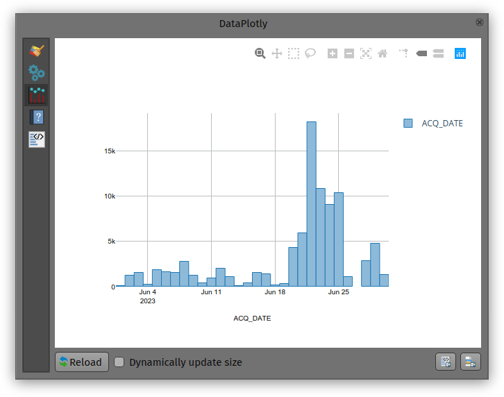
While not perfect, an histogram can quickly provide a good sense of a fire event’s “peak” over a period of time.

QField background tracking

Years ago, the QField community and its users showed their love for their favourite field app by supporting a successful crowdfunding to improve camera handling.

Since then, OPENGIS.ch has continued to lead the development of QField with the regular support of sponsors. We couldn’t be prouder of the progress we have made, with plenty of new features added in every major release. This includes major improvements to positioning including location tracking, integration of external GNSS receivers through not only Bluetooth but TCP/UDP and serial port connections, accuracy indicator and constraints, and most recently sensors reading to list a few.

We are now calling for the community to help further better QField and unlock an important milestone: background location tracking service.

Main goal: background location tracking on Android – 25’000€

Currently, QField requires users to keep their devices’ screen on and have the app in the foreground to keep track of the device’s positioning location. On mobile devices, this can drain batteries faster than many would want to, in environments where charging options are limited.

This crowdfunding aims at removing this constraint and allow QField – via a background service – to constantly keep tracking location even while the device is suspended (i.e., when the screen is turned off / locked). 

To achieve this, a significant amount of work is required as the positioning framework on Android will need to be relocated to a dedicated background service. Recent work we’ve done adding a background service to synchronize captured image attachments in QFieldCloud projects armed us with the assurances that we can achieve our goal while giving us an appreciation of the large amount of work needed.

Some of the benefits

Running out of battery is the nightmare of most field surveyors. By moving location tracking to a background service, users will be able to improve their battery life considerably and keep focusing on their tasks even if it involves switching to a different app.

Furthermore, while OPENGIS.ch ninjas remain busy squashing reported QField crashes all year long, there will always be unexpected scenarios leading to abrupt app shutdowns, such as third-party apps, systems running out of battery, etc. To address this, the background service framework will also act as a safeguard to avoid location data loss when QField unexpectedly shuts down and offer users means to recover that data upon re-opening QField.

Stretch goal 1: background navigation audio feedback 5’000€

The second stretch goal builds onto QField’s nice fly-to-point navigation system. If the QField community meets this threshold, a new background navigation audio feedback informing users in the field of their proximity to their target will be implemented. 

The audio feedback will use text-to-speech technology to state the distance to target in meters for a given time or distance interval.

Stretch goal 2: iOS 15’000€

The main goal will cover the Android implementation only. Due to being a very low level work we will have to replicate the work for each platform we support. If we reach stretch goal 2 we will also implement this for iOS.

Pledge now:

In case you do not see the embedded form you can open it directly here.

Thanks for supporting our crowdfunding and keep an eye on our blog for updates on the status.

How to contribute to QField

QField is a community-driven open-source project. It is free to share, use and modify and it will stay like that. The very essence of a community is to help and support each other. And that’s where YOU come into play. To make it work we need your support!

For those who don’t know much about the concept of open source projects, a bit of background. Investing in open-source projects is a technical and ethical decision for OPENGIS.ch. Open source is a technological advantage, as we receive input from many developers worldwide who are motivated to work out the best possible software. It prevents our customers from vendor lock-in and allows complete ownership and control of the developed software. And finally, not only financially independent businesses and people should benefit from professional software but also those who might not have the financial means to pay for features, and licences. 

You are not a developer, but you still like to use QField and support it? Good news. You don’t have to be a developer to use, contribute or recommend the app. There are plenty of things that need to be done to help QField to remain the powerful software it is right now and become even better. Here are a few suggestions on how you can give something back.

  1. Review the app ★★★★★ in google’s play store or apple’s app store
  2. Let the world know about it! It doesn’t matter if you’re on Twitter, LinkedIn, Instagram or any other social media platform. Show and tell about where QField helped you. We appreciate every post and we promise to like, share and comment.
  3. Write about your experience and please let us know. Be it in your blog or as a new success story. Insights into field projects are extremely valuable. It helps us to make the app even more efficient for your work, and it helps others to understand the range of applications for QField.
  4. Register for a paid QFieldCloud account. QFieldCloud allows to synchronize and merge the data collected in QField. QFieldCloud is hosted by the makers of QField and by getting an account you help QField too.

Do you want to do something that is more hands-on and directly linked to the app? No problem. 

  1. Help with the documentation. You can document features, or improve the documentation in English. Read the how-to guide to get started.
  2. And if you are multilingual you might consider translating the documentation or the app in your language.
  3. Become a beta tester and be the first to report a bug! When something doesn’t work properly it might be a bug. The quicker we know about it, the faster it can be resolved.
  4. You can ask and answer questions on gis.stackexchange and help others on the user discussions platform.
  5. If you are a developer and you want to get involved in QField development, please refer to the individual documentation for QField, QFieldCloud and QFieldSync.

And now finally for those of you who have the financial means, you can either sponsor a feature or subscribe to one of the monthly sponsorships. By doing so you help get freshly baked QField versions straight to everyone’s devices.

Nothing in it for you? In that case, just drop by to say thank you or have a hot or cold beverage with us next time you meet OPENGIS.ch at a conference and you might make our day!
Want to know more about the idea of community-driven open-source projects and the QGIS project in particular? Check out Nyall Dawson’s blog post about how to effectively get things done in open source!

QGIS Relations, their Widgets and the Plugins of them

This blog post is about QGIS relations and how they are edited in the attribute form with widgets in general, as well as some plugins that override the relations editor widget to improve usability and solve specific use cases. The start is quite basic. If you are already a relation hero, then jump directly to the plugins.

QGIS Relations in General

Let’s have a look at a simple example data model. We have four entities: Building, Apartment, Address and Owner. In UML it looks like this:

  • A building can have none or multiple apartments, but an apartment must to be related to a building. This black box on the left describes the relation strength as a composition. An apartment cannot exist without a building. When a building is demolished, all apartments of it are demolished as well.
  • An apartment needs to be owned by at least one owner. An owner can own none or more apartments. This is a many-to-many relation and this means, it will be normalized by adding a linking (join) table in between.
  • A building can have an address (only one – no multiple entrances in this example). An address can refer to one building.
    Why not making one single table on a one-to-one relation? To ensure their existence independently: When a building is demolished, the address should persist until the new building is constructed.

Creating Relations in QGIS

In QGIS we have now five layers. The four entities and the linking table called “Apartment_Owner”.

Open Project > Properties… > Relations

With Discover Relations the possible relations are detected from the existing layers according to their foreign keys in the database. In this example no CASCADE is defined in the database what means that the relations strength is always “Association”.

Where would “Composition” make sense?

Of course in the relation “Apartment” to “Building”, to ensure that when a feature of “Building” is deleted, the children (“Apartment”) are deleted as well, because they cannot exist without a building. Also a duplication of a feature of “Building” would duplicate the children (“Apartment”) as well.

But as well on the linking (join) table “Apartment_Owner” and its relation to “Apartment” and “Owner” a composition would make sense. Because when a feature of “Apartment” or “Owner” is deleted, the entry in the linking table should be deleted as well. Because this connection does not exist anymore and otherwise this would lead to orphan entries in the linking table.

Walk through the widgets

To demonstrate the relation widgets Relation EditorRelation Reference and Value Relation we make a walk through the digitizing process.

Relation Editor

First we create a “Building” and call it “Garden Tower”. Then we add some “Apartments”.

The “Apartments” are created in the widget called Relation Editor. This shows us a list (similar to the QGIS Attribute Table) of all children (“Apartment”) referencing to this “Building”. We have here activated the possibilities to adddelete and duplicate child-features.

In the widget settings (Right-click on the layer > Properties… > Attribute Form) we see that there are other possibilities to link and unlink child-features as well as zoom to the current child-feature (what only would make sense when they have a geometry).

As well we can set here the cardinality. This will become interesting when we go to the “Owner” to “Apartment” relation. But let’s first have a look at the opposite of what we just did.

Relation Reference

When we open now a feature of “Apartment”, we see that we have a drop down to select the “Building” to reference to.

On the right of this drop down we can see some buttons. Those are for the following functionalities (from left to right):

  • Open the form of the current parent feature (in our case the “Building” feature called “Garden Tower”)
  • Add a new feature on the parent layer (in our case “Building”)
  • Highlight the parent layer (in our case “Building”) on the map
  • Select the parent feature (in our case “Building”) on the map to reference it

In the settings (Right-click on the layer > Properties… > Attribute Form) we see that we choose the configured relation to connect the child (“Apartment”) to the parent (“Building”). This won’t be needed with the widget Value Relation.

Value Relation

The Value Relation does not require a relation at all. We simply choose the “parent” layer (“Building”) its primary key as the key (“t_id”) and a descriptive field as the value (“Description”).

The result shows us a drop down as well to select the parent.

It is much easier to configure, but you can see the limitations. There are no such functionalities to control the parent feature like addidentify on map etc. As well you need to be careful to fulfill the foreign key constraint (you have to choose the correct field to link with). All this is given, when you build a Relation Reference on an existing relation.

Many-to-Many Relations

Now we link some “Owner” to our “Apartment”. We could create new ones like we did it for the “Apartment” in “Building” or we can link existing ones. For linking we choose the yellow link-button on the top of the Relation Editor.

This dialog looks similar to the Relation Editor widget. You have just to select the “Owner” you want to link to the “Apartment” by checking the yellow box. It’s a very powerful tool, but people are often confused about the load of functionality here and the selection that can be difficult to get used to (yellow boxes vs. blue index selection). For this case we extended the Relation Editor widget with a plugin.

Anyway after that we linked our features of the layer “Owner”.

Have you seen the linking table in between? Well, me neither. It’s completely invisible for the end user. This because of the cardinality setting I mentioned already. When we choose the linked table “Owner” instead of “Many to one relation”, then we can create and link the other parent (“Owner”) directly.

One-to-One Relation

A one-to-one relation like we have here between “Building” and “Address” is created in the database more or less like a normal one-to-many relation. This means one of the tables (in our case “Address”) has a foreign key pointing to the parent table (“Building”). There are tricks to fulfill the one-to-one maximum cardinality (like e.g. by setting a UNIQUE constraint on this foreign key column) but still in the QGIS user interface it looks like a one-to-many relation. It’s displayed in a normal Relation Editor widget.

Solutions could be so called “Joins”. Go to the settings (Right-click on the layer > Properties… > Joins)

Here you can join a layer of your choice and add the fields of this other layer (in our case “Address”) to your current feature form (of “Building”). So it appears to the user that it’s the same table containing fields of “Building” and “Address”.

Negative point about those joins are, that they are fault prone. You have to be careful with default values (e.g. on primary keys) of the joined layer. You cannot expect a fully reliable feature form like you have it in the Relation Editor. Here as well, we extended the Relation Editor widget with a plugin.

Plugins for Relation Editor Widgets

Since QGIS 3.18 the base class of the Relation Editor Widgets became abstract, what opened the possibility to use it in PyQGIS and derive it to super nice widgets handling specific use cases and improving the usability.

Linking Relation Editor Widget

As mentioned before, the QGIS stock dialog to link children is full of features but it can be overwhelming and difficult to use. Mostly because of the two selection possibilities in the list. A blue selection is for the currently displayed feature, and a yellow checkbox selection is for the features to be actually linked.

In collaboration with the Model Baker Group we wanted to improve the situation. But as we where unsure how the end solution should look like, so we decided to experiment in a plugin. The result is a link manger dialog, in which features can be linked and unlinked by moving them left and right. The effective link is created or destroyed when the dialog is accepted.

Find more information on the repository https://github.com/opengisch/qgis-linking-relation-editor

Ordered Relation Editor Widget

Sometimes the order of the children play a role on the project, and you want to have them displayed following that. For that there is the Ordered Relation Editor Widget. You can configure a field in the children to be used to order them. In the given example the field Floor was used to order Apartments. Reordering the fields by Drag&Drop would change the value of the configured field. Display name and optionally a path to an icon to be shown on the list can be configured by expression in the Attribute Form tab in the layer properties (Right-click on the layer > Properties… > Attribute Form).

Find more information on the repository https://github.com/opengisch/qgis-ordered-relation-editor

Document Management System Widgets

Often in QGIS projects there is the need to deal with external documents. This could be for example pictures, documentations or reports about some features. To support that we added two new tables in the project:

  • Documents each document is represented by a row in this table. The table has following fields:
    • id
    • path is the filename of the document.
  • DocumentsFeatures this is a linking (join) table and permits to link a document with one or more features in more layers. The table has following fields:
    • id
    • document_id id of the document.
    • feature_id id of the feature.
    • feature_layer layer of the feature.

Thanks to a QGIS feature named Polymorphic Relations we can link a document with features of multiple layers. The polymorphic relation can evaluate an expression to decide in which table will be the feature to link. Here a screenshot of the relation configuration:

After this configuration in the layers “Apartment” and “Building” it will be possible to link children from the “Documents” table. The document management plugin provides two widgets to simplify the handling of the relation. In the feature side widget the documents are displayed as a grid or list. If possible a preview of the contend is shown and you can add new documents via Drag&Drop from the system file manager. Double-click on a document will open it in the default system viewer.

The second widget is meant to be used in the Feature Form of the “Documents” table, and it permits to handy see, for each document, with which feature from which layer it is linked.

Find more information on the repository https://github.com/opengisch/qgis-document-management-system-plugin

That’s it

Well then. We hope that all the beginners reading this article received some light on QGIS Relations and all the advanced user some inspiration on the immense possibilities you have with QGIS ?

A New Trick up QField’s Sleeve: Animated Maps

Starting with QField 2.2, users can fully rely on animation capabilities that have made their way into QGIS during its last development cycle. This can be a powerful mean to highlight key elements on a map that require special user attention.

The example below demonstrates a scenario where animated raster markers are used to highlight active fires within the visible map extent. Notice how the subtle fire animation helps draw viewers’ eyes to those important markers.

Animated raster markers is a new symbol layer type in QGIS 3.26 that was developed by Nyall Dawson. Supported image formats include GIF, WEBP, and APNG.

The second example below showcases more advanced animated symbology which relies on expressions to animate several symbol properties such as marker size, border width, and color opacity. While more complex than simply adding a GIF marker, the results achieved with data-defined properties animation can be very appealing and integrate perfectly with any type of project.

You’ll quickly notice how smooth the animation runs. That is thanks to OPENGIS.ch’s own ninjas having spent time improving the map canvas element’s handling of layers constantly refreshing. This includes automatic skipping of frames on older devices so the app remains responsive.

Oh, we couldn’t help ourselves but take the opportunity to demonstrate how nice the QField feature form layout is these days in the video above 😄 To know more about other new features in QField 2.2, go and read the release page.

Happy field mapping to all!

The lovely animal markers used in the zoo example above were made by Serbian artist Arsenije Vujovic.

High Efficiency with Buffered Transactional Editing in QGIS

Tired of start/stop editing for every single layer in your project with mixed data sources?
Starting from version 3.26, QGIS has a new transaction mode called “Buffered Transaction Groups”.

Within this mode, all layers which are not read-only are put in one “transaction group” and handled together when the actions “Toggle Editing” or “Save Layer Edits” are activated. It doesn’t matter if the layers come from different providers like GeoPackage, PostgreSQL or Shapefile. Edits are buffered locally and saved within one single transaction on all layers per provider. With this, you can store all edited layers with a single click. And in comparison to the well-known “Automatic Transaction Groups” mode you have better performance during editing and fewer problems with locking of the database when multiple users edit the same table in parallel.

To try it out; go to Project -> Properties -> Data Sources -> Transaction mode

Enjoy and let us know what you think!

Limitations:

In databases, transactions are atomic. That is, the data can be completely and correctly written, or it will be completely rolled back. With buffered transactions, QGIS tries to do the same but has less control. When writing to different providers it could happen that, if an error occurs when writing to PostgreSQL, but some data were already written in a Shapefile the rollback will be only partial. This only applies to data from different data sources.

This feature was sponsored by Canton Glarus.

Writing a feature-based processing algorithm at the example of M-value interpolation

Amongst all the processing algorithms already available in QGIS, sometimes the one thing you need is missing. 

This happened not a long time ago, when we were asked to find a way to continuously visualise traffic on the Swiss motorway network (polylines) using frequently measured traffic volumes from discrete measurement stations (points) alongside the motorways. In order to keep working with the existing polylines, and be able to attribute more than one value of traffic to each feature, we chose to work with the M-values. M-values are a per-vertex attribute like X, Y or Z coordinates. They contain a measure value, which typically represents time or distance. But they can hold any numeric value.

In our example, traffic measurement values are provided on a separate point layer and should be attributed to the M-value of the nearest vertex of the motorway polylines. Of course, the motorway features should be of type LineStringM in order to hold an M-value. We then should interpolate the M-values for each feature over all vertices in order to get continuous values along the line (i.e. a value on every vertex). This last part is not yet existing as a processing algorithm in QGIS.

This article describes how to write a feature-based processing algorithm based on the example of M-value interpolation along LineStrings.

Feature-based processing algorithm

The pyqgis class QgsProcessingFeatureBasedAlgorithm is described as follows: “An abstract QgsProcessingAlgorithm base class for processing algorithms which operates “feature-by-feature”.  

Feature based algorithms are algorithms which operate on individual features in isolation. These are algorithms where one feature is output for each input feature, and the output feature result for each input feature is not dependent on any other features present in the source. […]

Using QgsProcessingFeatureBasedAlgorithm as the base class for feature based algorithms allows shortcutting much of the common algorithm code for handling iterating over sources and pushing features to output sinks. It also allows the algorithm execution to be optimised in future (for instance allowing automatic multi-thread processing of the algorithm, or use of the algorithm in “chains”, avoiding the need for temporary outputs in multi-step models).

In other words, when connecting several processing algorithms one after the other – e.g. with the graphical modeller – these feature-based processing algorithms can easily be used to fill in the missing bits. 

Compared to the standard QgsProcessingAlgorithm the feature-based class implicitly iterates over each feature when executing and avoids writing wordy loops explicitly fetching and applying the algorithm to each feature. 

Just like for the QgsProcessingAlgorithm (a template can be found in the Processing Toolbar > Scripts > Create New Script from Template), there is quite some boilerplate code in the QgsProcessingFeatureBasedAlgorithm. The first part is identical to any QgsProcessingAlgorithm.

After the description of the algorithm (name, group, short help, etc.), the algorithm is initialised with def initAlgorithm, defining input and output. 

In our M-value example:

    def initAlgorithm(self, config=None):
        self.addParameter(
            QgsProcessingParameterFeatureSource(
                self.INPUT,
                self.tr('Input layer'),
                [QgsProcessing.TypeVectorAnyGeometry]
            )
        )
        self.addParameter(
            QgsProcessingParameterFeatureSink(
                self.OUTPUT,
                self.tr('Output layer')
            )
        )

While in a regular processing algorithm now follows def processAlgorithm(self, parameters, context, feedback), in a feature-based algorithm we use def processFeature(self, feature, context, feedback). This implies applying the code in this block to each feature of the input layer. 

! Do not use def processAlgorithm in the same script, otherwise your feature-based processing algorithm will not work !

Interpolating M-values

This actual processing part can be copied and added almost 1:1 from any other independent python script, there is little specific syntax to make it a processing algorithm. Only the first line below really.

In our M-value example:

    def processFeature(self, feature, context, feedback):
        
        try:
            geom = feature.geometry()
            line = geom.constGet()
            vertex_iterator = QgsVertexIterator(line)
            vertex_m = []

            # Iterate over all vertices of the feature and extract M-value

            while vertex_iterator.hasNext():
                vertex = vertex_iterator.next()
                vertex_m.append(vertex.m())

            # Extract length of segments between vertices

            vertices_indices = range(len(vertex_m))
            length_segments = [sqrt(QgsPointXY(line[i]).sqrDist(QgsPointXY(line[j]))) 
                for i,j in itertools.combinations(vertices_indices, 2) 
                if (j - i) == 1]

            # Get all non-zero M-value indices as an array, where interpolations 
              have to start

            vertex_si = np.nonzero(vertex_m)[0]
            
            m_interpolated = np.copy(vertex_m)

            # Interpolate between all non-zero M-values - take segment lengths between 
              vertices into account

            for i in range(len(vertex_si)-1):
                first_nonzero = vertex_m[vertex_si[i]]
                next_nonzero = vertex_m[vertex_si[i+1]]
                accum_dist = itertools.accumulate(length_segments[vertex_si[i]
                                                                  :vertex_si[i+1]])
                sum_seg = sum(length_segments[vertex_si[i]:vertex_si[i+1]])
                interp_m = [round(((dist/sum_seg)*(next_nonzero-first_nonzero)) + 
                            first_nonzero,0) for dist in accum_dist]
                m_interpolated[vertex_si[i]:vertex_si[i+1]] = interp_m

            # Copy feature geometry and set interpolated M-values, 
              attribute new geometry to feature

            geom_new = QgsLineString(geom.constGet())
            
            for j in range(len(m_interpolated)):
                geom_new.setMAt(j,m_interpolated[j])
                
            attrs = feature.attributes()
            
            feat_new = QgsFeature()
            feat_new.setAttributes(attrs)
            feat_new.setGeometry(geom_new)

        except Exception:
            s = traceback.format_exc()
            feedback.pushInfo(s)
            self.num_bad += 1
            return []
        
        return [feat_new]

In our example, we get the feature’s geometry, iterate over all its vertices (using the QgsVertexIterator) and extract the M-values as an array. This allows us to assign interpolated values where we don’t have M-values available. Such missing values are initially set to a value of 0 (zero).

We also extract the length of the segments between the vertices. By gathering the indices of the non-zero M-values of the array, we can then interpolate between all non-zero M-values, considering the length that separates the zero-value vertex from the first and the next non-zero vertex.

For the iterations over the vertices to extract the length of the segments between them as well as for the actual interpolation between all non-zero M-value vertices we use the library itertools. This library provides different iterator building blocks that come in quite handy for our use case. 

Finally, we create a new geometry by copying the one which is being processed and setting the M-values to the newly interpolated ones.

And that’s all there is really!

Alternatively, the interpolation can be made using the interp function of the numpy library. Some parts where our manual method gave no values, interp.numpy seemed more capable of interpolating. It remains to be judged which version has the more realistic results.

Styling the result via M-values

The last step is styling our output layer in QGIS, based on the M-values (our traffic M-values are categorised from 1 [a lot of traffic -> dark red] to 6 [no traffic -> light green]). This can be achieved by using a Single Symbol symbology with a Marker Line type “on every vertex”. As a marker type, we use a simple round point. Stroke style is “no pen” and Stroke fill is based on an expression:

with_variable(

'm_value', m(point_n($geometry, @geometry_point_num)),

	CASE WHEN @m_value = 6
		THEN color_rgb(140, 255, 159)

		WHEN @m_value = 5
			THEN color_rgb(244, 252, 0)

		WHEN @m_value = 4
			THEN color_rgb(252, 176, 0)

		WHEN @m_value = 3
			THEN color_rgb(252, 134, 0)

		WHEN @m_value = 2
			THEN color_rgb(252, 29, 0)

		WHEN @m_value = 1
			THEN color_rgb(140, 255, 159)

		ELSE
			color_hsla(0,100,100,0)

	END
)

And voilà! Wherever we have enough measurements on one line feature, we get our motorway network continuously coloured according to the measured traffic volume.

One disclaimer at the end: We get this seemingly continuous styling only because of the combination of our “complex” polylines (containing many vertices) and the zoomed-out view of the motorway network. Because really, we’re styling many points and not directly the line itself. But in our case, this is working very well.

If you’d like to make your custom processing algorithm available through the processing toolbox in your QGIS, just put your script in the folder containing the files related to your user profile:

profiles > default > processing > scripts 

You can directly access this folder by clicking on Settings > User Profiles > Open Active Profile Folder in the QGIS menu.

That way, it’s also available for integration in the graphical modeller.

Extract of the Graphical Modeler sequence. “Interpolate M-values neg” refers to the custom feature-based processing algorithm described above.


You can download the above-mentioned processing scripts (with numpy and without numpy) here.

Happy processing!

QField 1.9 Taivaskero is out to further empower users

From unlocking selective atlas layout export to opening individual datasets and creating GeoPDFs, QField 1.9 is all about giving even more power to its users. The release also comes with significant user experience improvement, such as faster rendering and restoring the last viewed map extent.

Print Atlas-Driven Layouts to PDF

QField has long supported exporting print layouts to PDF, but now users are able to export atlas-driven layouts from selected features, all while being in the field. A new print action is now attached to the feature form and identified features list for all vector layers acting as atlas coverage layers in any of the print layouts present in a loaded project.

Oh, and did we mention exported PDFs from QField are now georeferenced?

Opening of individual datasets

Users in the field can find themselves in need of opening individual geospatial datasets not bound to a project: that KML file a colleague has just sent through via a messenger app or a new GeoPDF sitting in the inbox. QField 1.9 will seamlessly do that for you.

geopackage

Out of the box, users will now be able to open vector and rasters datasets from their mobile devices. By default, an OpenStreetMap base map will be added as an underlying basemap to the opened dataset layer(s).

Geometry digitizing when adding child features to relationships

While QField has long allowed users to add new child features to predefined layers’ relationships, users were only able to add feature attributes. This changes with this new version of QField.

As of now, users will be able to digitize geometries alongside attributes for new child features. This is a significant user experience improvement and will surely ease field data entry in many cases.

A maturing search bar now with address searches

A new address search framework was added to QField’s search bar. In this new version, Finnish users will be able to search for street addresses and locations straight from QField. More coverage is planned in future releases.

serach

If you want to sponsor a specific country, contact us.

User interface and experience improvements

While this new version of QField brings an exciting amount of new features, it also showcases countless refinements and improvements to its user interface and experience. Some noteworthy improvements include:

  • QField now remembers the last map extent for each project and dataset opened, allowing users to launch QField and pick things up where they left off.
  • QField now provides visual feedback when opening large projects so users don’t have to wonder what is happening to a frozen QField frame.
  • Significant attention was paid to improve the visual consistency of the feature form widgets, and users will be pleased to see project-set background colours for attributes are now reflected in the QField interface.

QField Cloud

We have also been working hard on improved methods for synchronizing data from field to the office. QField Cloud is looming around the corner to help you simplify processes and data integration. Don’t miss out and join the waiting list if you haven’t done so already!

That’s it! Thanks for reading and check out the complete changelog on our repository.

Generate DXF on QGIS server

Everyone knows QGIS is on the desktop and mobile devices. Many know QGIS is on the web with QGIS server through OGC services. Some know QGIS server has its own extension to generate PDFs. But did you know that QGIS server can also produce DXF files?

DXF

DXF files are mainly used for interchanging CAD drawings, vector geometries with styles and attributes. With a couple of compromises, these files can be imported and exported to and from QGIS.

Due to their heavy use of CAD software, architects work a lot with DXF files. For example, for the Swiss Cadastral Survey (Amtliche Vermessung, Mensuration Officielle) there is a standard with the name GEOBAU-DXF that defines layer names and structure of this file. Architects often request this format from cantonal government agencies when planning construction work.

In the canton of Schaffhausen, there are over 100 downloads per month and it’s by far the most demanded format. These files were produced semi-automatically through a separate application and the customers got the data by mail with a link to a zip file. The time between order and delivery was about 20 minutes. With the renewal of the cantonal SDI, including QGIS server for handling OGC services, the situation changed and an update to this process was required.

Optimize the process

For the canton of Schaffhausen, the goal was to find a solution with existing components of the new SDI, completely based on machine-to-machine communication and to make the turnaround time for the customer as fast as possible. As soon as they realized QGIS server is also able to deliver DXF, this seemed to be the best approach to fulfil their needs concerning the download of GEOBAU-DXF. And, with the help of OPENGIS.ch, it was a full success.

In the cantonal infrastructure, the data is available in a Postgres database, which is regularly filled through an ETL workflow. On top of this database, the canton created a QGIS project with symbology, labelling and layers that reflect the GEOBAU-DXF standard.

With this project published on a QGIS server, it was quickly possible to generate a DXF file, but some improvements were still required in QGIS 3.10.

  • Label alignment was not preserved
  • Altitudes (Z values) of coordinates were not properly exported
  • Symbols were defined inline and not in blocks
  • When a layer could have mixed geometry types (points, lines and polygons) there were problems with missing objects and wrong symbology

The Canton Shaffausen already had a support and maintenance contract in place with us and used this contract to kick off the development as well as requesting an additional dedicated development contract with specific goals. A couple of iterations later these enhancements were released with the next QGIS versions and are now available for everyone.

As a side effect, the DXF code has been cleaned up. This is now in a much more solid and modular state (it would, for example, be straightforward to expose it as processing algorithm now). Another nice improvement was that QGIS WMS server is now able to handle multiple layers with the same name, merging them to a single layer. This can be interesting if you have to expose the same layer multiple times with points, lines and polygons.

Meanwhile in Schaffhausen, the service is running in production and architects can happily obtain DXF-GEOBAU files by choosing the area of interest on the web map and download the file in no time.

To try it out, head over to the geoportal of the canton of Schaffhausen, click the three-dots menu and choose GEOBAU-DXF.

Or directly use the following download sample link to generate a GEOBAU-DXF file: https://wfs.geo.sh.ch/dxfgeobau?SERVICE=WMS&VERSION=1.3.0&REQUEST=GetMap&LAYERS=dxfgeobau&STYLES=&CRS=EPSG%3A2056&BBOX=2690035,1283484,2690299,1283694&WIDTH=1042&HEIGHT=811&FORMAT_OPTIONS=MODE:SYMBOLLAYERSYMBOLOGY;SCALE:500;NO_MTEXT:TEXT&FILE_NAME=geobau.dxf&FORMAT=application/dxf

  • Page 1 of 1 ( 9 posts )
  • uncategorised

Back to Top

Sustaining Members