Related Plugins and Tags

QGIS Planet

Mapping relationships between Neo4j spatial nodes with GeoPandas

Previously, we mapped neo4j spatial nodes. This time, we want to take it one step further and map relationships.

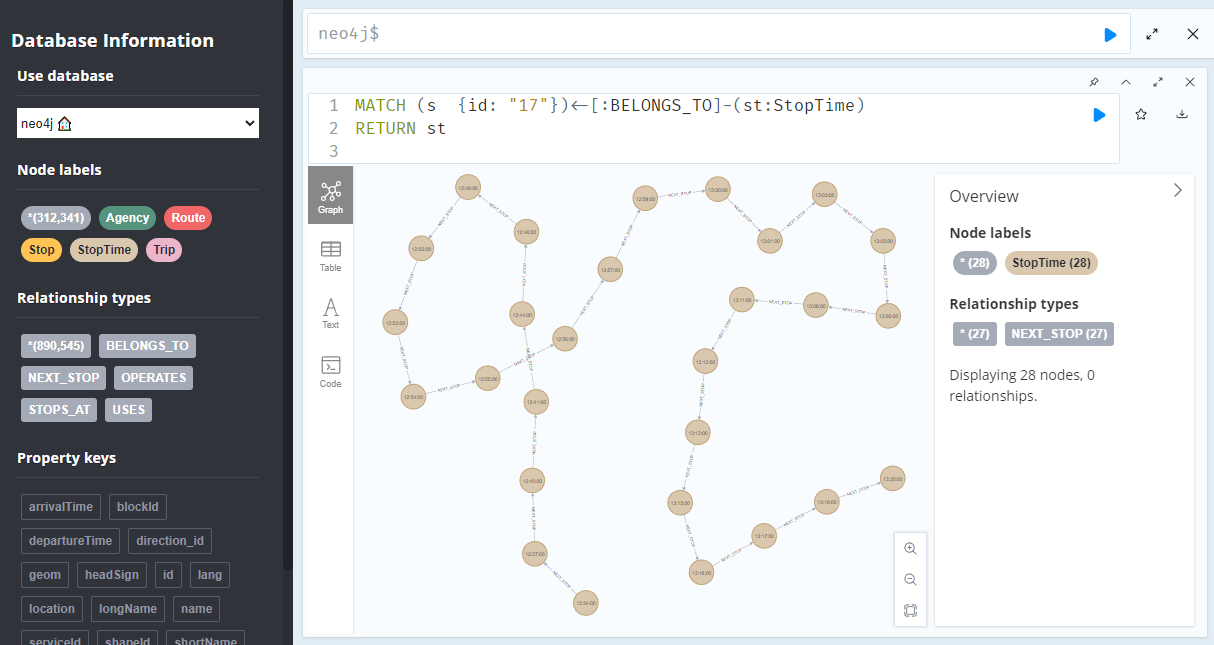
A prime example, are the relationships between GTFS StopTime and Trip nodes. For example, this is the Cypher query to get all StopTime nodes of Trip 17:

MATCH 
    (t:Trip  {id: "17"})
    <-[:BELONGS_TO]-
    (st:StopTime) 
RETURN st

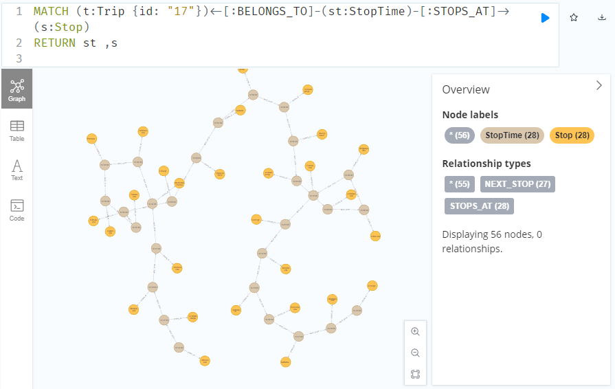
To get the stop locations, we also need to get the stop nodes:

MATCH 
    (t:Trip {id: "17"})
    <-[:BELONGS_TO]-
    (st:StopTime)
    -[:STOPS_AT]->
    (s:Stop)
RETURN st ,s

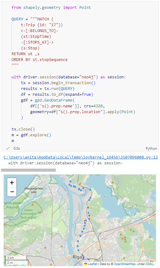
Adapting our code from the previous post, we can plot the stops:

from shapely.geometry import Point

QUERY = """MATCH (
    t:Trip {id: "17"})
    <-[:BELONGS_TO]-
    (st:StopTime)
    -[:STOPS_AT]->
    (s:Stop)
RETURN st ,s
ORDER BY st.stopSequence
"""

with driver.session(database="neo4j") as session:
    tx = session.begin_transaction()
    results = tx.run(QUERY)
    df = results.to_df(expand=True)
    gdf = gpd.GeoDataFrame(
        df[['s().prop.name']], crs=4326,
        geometry=df["s().prop.location"].apply(Point)
    )

tx.close() 
m = gdf.explore()
m

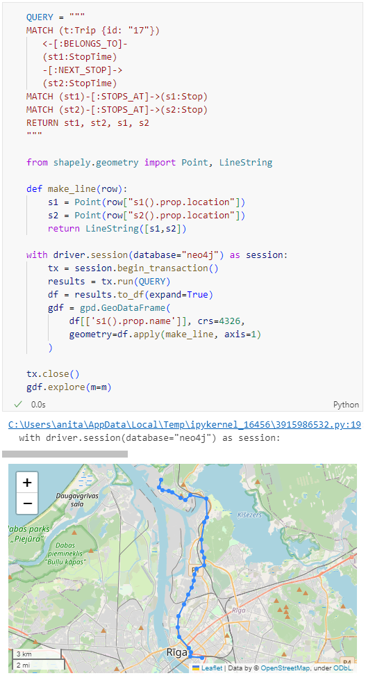
Ordering by stop sequence is actually completely optional. Technically, we could use the sorted GeoDataFrame, and aggregate all the points into a linestring to plot the route. But I want to try something different: we’ll use the NEXT_STOP relationships to get a DataFrame of the start and end stops for each segment:

QUERY = """
MATCH (t:Trip {id: "17"})
   <-[:BELONGS_TO]-
   (st1:StopTime)
   -[:NEXT_STOP]->
   (st2:StopTime)
MATCH (st1)-[:STOPS_AT]->(s1:Stop)
MATCH (st2)-[:STOPS_AT]->(s2:Stop)
RETURN st1, st2, s1, s2
"""

from shapely.geometry import Point, LineString

def make_line(row):
    s1 = Point(row["s1().prop.location"])
    s2 = Point(row["s2().prop.location"])
    return LineString([s1,s2])

with driver.session(database="neo4j") as session:
    tx = session.begin_transaction()
    results = tx.run(QUERY)
    df = results.to_df(expand=True)
    gdf = gpd.GeoDataFrame(
        df[['s1().prop.name']], crs=4326,
        geometry=df.apply(make_line, axis=1)
    )

tx.close() 
gdf.explore(m=m)

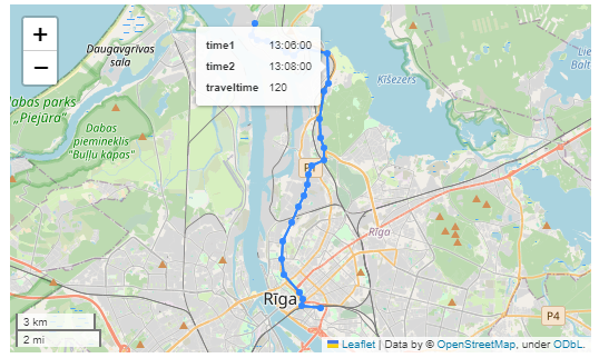
Finally, we can also use Cypher to calculate the travel time between two stops:

MATCH (t:Trip {id: "17"})
   <-[:BELONGS_TO]-
   (st1:StopTime)
   -[:NEXT_STOP]->
   (st2:StopTime)
MATCH (st1)-[:STOPS_AT]->(s1:Stop)
MATCH (st2)-[:STOPS_AT]->(s2:Stop)
RETURN st1.departureTime AS time1, 
   st2.arrivalTime AS time2, 
   s1.location AS geom1, 
   s2.location AS geom2, 
   duration.inSeconds(
      time(st1.departureTime), 
      time(st2.arrivalTime)
   ).seconds AS traveltime

As always, here’s the notebook: https://github.com/anitagraser/QGIS-resources/blob/master/qgis3/notebooks/neo4j.ipynb

Adding basemaps to PyQGIS maps in Jupyter notebooks

In the previous post, we investigated how to bring QGIS maps into Jupyter notebooks.

Today, we’ll take the next step and add basemaps to our maps. This is trickier than I would have expected. In particular, I was fighting with “invalid” OSM tile layers until I realized that my QGIS application instance somehow lacked the “WMS” provider.

In addition, getting basemaps to work also means that we have to take care of layer and project CRSes and on-the-fly reprojections. So let’s get to work:

from IPython.display import Image
from PyQt5.QtGui import QColor
from PyQt5.QtWidgets import QApplication
from qgis.core import QgsApplication, QgsVectorLayer, QgsProject, QgsRasterLayer, \
    QgsCoordinateReferenceSystem, QgsProviderRegistry, QgsSimpleMarkerSymbolLayerBase
from qgis.gui import QgsMapCanvas
app = QApplication([])
qgs = QgsApplication([], False)
qgs.setPrefixPath(r"C:\temp", True)  # setting a prefix path should enable the WMS provider
qgs.initQgis()
canvas = QgsMapCanvas()
project = QgsProject.instance()
map_crs = QgsCoordinateReferenceSystem('EPSG:3857')
canvas.setDestinationCrs(map_crs)
print("providers: ", QgsProviderRegistry.instance().providerList())

To add an OSM basemap, we use the xyz tiles option of the WMS provider:

urlWithParams = 'type=xyz&url=https://tile.openstreetmap.org/{z}/{x}/{y}.png&zmax=19&zmin=0&crs=EPSG3857'
rlayer = QgsRasterLayer(urlWithParams, 'OpenStreetMap', 'wms')  
print(rlayer.crs())
if rlayer.isValid():
    project.addMapLayer(rlayer)
else:
    print('invalid layer')
    print(rlayer.error().summary()) 

If there are issues with the WMS provider, rlayer.error().summary() should point them out.

With both the vector layer and the basemap ready, we can finally plot the map:

canvas.setExtent(rlayer.extent())
plot_layers([vlayer,rlayer])

Of course, we can get more creative and style our vector layers:

vlayer.renderer().symbol().setColor(QColor("yellow"))
vlayer.renderer().symbol().symbolLayer(0).setShape(QgsSimpleMarkerSymbolLayerBase.Star)
vlayer.renderer().symbol().symbolLayer(0).setSize(10)
plot_layers([vlayer,rlayer])

And to switch to other basemaps, we just need to update the URL accordingly, for example, to load Carto tiles instead:

urlWithParams = 'type=xyz&url=http://basemaps.cartocdn.com/dark_all/{z}/{x}/{y}.png&zmax=19&zmin=0&crs=EPSG3857'
rlayer2 = QgsRasterLayer(urlWithParams, 'Carto', 'wms')  
print(rlayer2.crs())
if rlayer2.isValid():
    project.addMapLayer(rlayer2)
else:
    print('invalid layer')
    print(rlayer2.error().summary()) 
    
plot_layers([vlayer,rlayer2])

You can find the whole notebook at: https://github.com/anitagraser/QGIS-resources/blob/master/qgis3/notebooks/basemaps.ipynb

PyQGIS Jupyter notebooks on Windows using Conda

The QGIS conda packages have been around for a while. One of their use cases, for example, is to allow Linux users to easily install multiple versions of QGIS.

Similarly, we’ve seen posts on using PyQGIS in Jupyter notebooks. However, I find the setup with *.bat files rather tricky.

This post presents a way to set up a conda environment with QGIS that is ready to be used in Jupyter notebooks.

The first steps are to create a new environment and install QGIS. I use mamba for the installation step because it is faster than conda but you can use conda as well:

(base) PS C:\Users\anita> conda create -n qgis python=3.9
(base) PS C:\Users\anita> conda activate qgis
(qgis) PS C:\Users\anita> mamba install -c conda-forge qgis=3.28.2 
(qgis) PS C:\Users\anita> qgis

If we now try to import the qgis module in Python, we get an error:

(qgis) PS C:\Users\anita> python
Python 3.9.15 | packaged by conda-forge | (main, Nov 22 2022, 08:41:22) [MSC v.1929 64 bit (AMD64)] on win32
Type "help", "copyright", "credits" or "license" for more information.
>>> import qgis
Traceback (most recent call last):
  File "<stdin>", line 1, in <module>
ModuleNotFoundError: No module named 'qgis'

To fix this error, we need to get the paths from the Python console inside QGIS:

import sys
sys.path
['H:/miniconda3/envs/qgis/Library/./python', 'C:/Users/anita/AppData/Roaming/QGIS/QGIS3\\profiles\\default/python', ... ]

This list of paths can be configured as the defaults for our qgis environment using conda develop:

(qgis) PS C:\Users\anita> conda activate base
(base) PS C:\Users\anita> mamba install conda-build -c conda-forge
(base) PS C:\Users\anita> conda develop -n qgis [list of paths from qgis python console] 

With this setup, the import should now work without errors:

(base) PS C:\Users\anita> conda activate qgis
(qgis) PS C:\Users\anita> python
Python 3.9.15 | packaged by conda-forge | (main, Nov 22 2022, 08:41:22) [MSC v.1929 64 bit (AMD64)] on win32
Type "help", "copyright", "credits" or "license" for more information.
>>> import qgis

The example Jupyter notebook covers running a QGIS Processing algorithm and visualizing the results in the notebook using GeoPandas:

Head over to Github to find the full instructions: https://github.com/anitagraser/QGIS-resources/blob/master/qgis3/notebooks/hello-world.ipynb

Building an interactive app with geocoding in Jupyter Lab

This post aims to show you how to create quick interactive apps for prototyping and data exploration using Panel.

Specifically, the following example demos how to add geocoding functionality based on Geopy and Nominatim. As such, this example brings together tools we’ve previously touched on in Super-quick interactive data & parameter exploration and Geocoding with Geopy.

Here’s a quick preview of the resulting app in action:

To create this app, I defined a single function called my_plot which takes the address and desired buffer size as input parameters. Using Panel’s interact and servable methods, I’m then turning this function into the interactive app you’ve seen above:

import panel as pn
from geopy.geocoders import Nominatim
from utils.converting import location_to_gdf
from utils.plotting import hvplot_with_buffer

locator = Nominatim(user_agent="OGD.AT-Lab")

def my_plot(user_input="Giefinggasse 2, 1210 Wien", buffer_meters=1000):
    location = locator.geocode(user_input)
    geocoded_gdf = location_to_gdf(location, user_input)
    map_plot = hvplot_with_buffer(geocoded_gdf, buffer_meters, 
                                  title=f'Geocoded address with {buffer_meters}m buffer')
    return map_plot.opts(active_tools=['wheel_zoom']) 

kw = dict(user_input="Giefinggasse 2, 1210 Wien", buffer_meters=(0,10000))

pn.template.FastListTemplate(
    site="Panel", title="Geocoding Demo", 
    main=[pn.interact(my_plot, **kw)]
).servable();

You can find the full notebook in the OGD.AT Lab repository or run this notebook directly on MyBinder:

To open the Panel preview, press the green Panel button in the Jupyter Lab toolbar:

I really enjoy building spatial data exploration apps this way, because I can start off with a Jupyter notebook and – once I’m happy with the functionality – turn it into a pretty app that provides a user-friendly exterior and hides the underlying complexity that might scare away stakeholders.

Give it a try and share your own adventures. I’d love to see what you come up with.

  • Page 1 of 1 ( 4 posts )
  • jupyter

Back to Top

Sustaining Members