Related Plugins and Tags

QGIS Planet

Analyzing video-based bicycle trajectories

Did you know that MovingPandas also supports local image coordinates? Indeed, it does.

In today’s post, we will explore how we can use this feature to analyze bicycle tracks extracted from video footage published by Michael Szell @mszll:

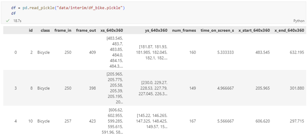
The bicycle trajectory coordinates are stored in two separate lists: xs_640x360 and ys640x360:

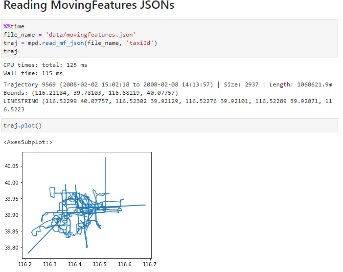
This format is kind of similar to the Kaggle Taxi dataset, we worked with in the previous post. However, to use the solution we implemented there, we need to combine the x and y coordinates into nice (x,y) tuples:

df['coordinates'] = df.apply(
    lambda row: list(zip(row['xs_640x360'], row['ys_640x360'])), axis=1)
df.drop(columns=['xs_640x360', 'ys_640x360'], inplace=True)

Afterwards, we can create the points and compute the proper timestamps from the frame numbers:

def compute_datetime(row):
    # some educated guessing going on here: the paper states that the video covers 2021-06-09 07:00-08:00
    d = datetime(2021,6,9,7,0,0) + (row['frame_in'] + row['running_number']) * timedelta(seconds=2)
    return d
def create_point(xy):
    try: 
        return Point(xy)
    except TypeError:  # when there are nan values in the input data
        return None
new_df = df.head().explode('coordinates')
new_df['geometry'] = new_df['coordinates'].apply(create_point)
new_df['running_number'] = new_df.groupby('id').cumcount()
new_df['datetime'] = new_df.apply(compute_datetime, axis=1)
new_df.drop(columns=['coordinates', 'frame_in', 'running_number'], inplace=True)
new_df

Once the points and timestamps are ready, we can create the MovingPandas TrajectoryCollection. Note how we explicitly state that there is no CRS for this dataset (crs=None):

trajs = mpd.TrajectoryCollection(
    gpd.GeoDataFrame(new_df), 
    traj_id_col='id',  t='datetime', crs=None)

Plotting trajectories with image coordinates

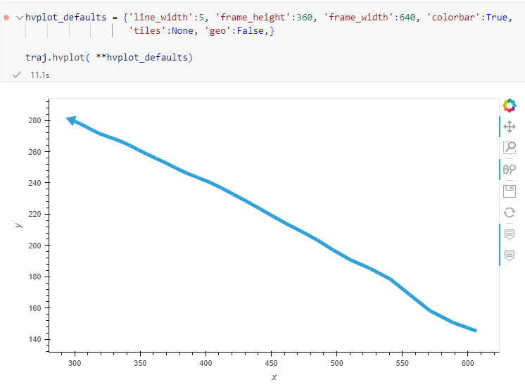
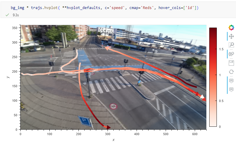
Similarly, to plot these trajectories, we should tell hvplot that it should not fetch any background map tiles (’tiles’:None) and that the coordinates are not geographic (‘geo’:False):

If you want to explore the full source code, you can find my Github fork with the Jupyter notebook at: https://github.com/anitagraser/desirelines/blob/main/mpd.ipynb

The repository also contains a camera image of the intersection, which we can use as a background for our trajectory plots:

bg_img = hv.RGB.load_image('img/intersection2.png', bounds=(0,0,640,360)) 

One important caveat is that speed will be calculated in pixels per second. So when we plot the bicycle speed, the segments closer to the camera will appear faster than the segments in the background:

To fix this issue, we would have to correct for the distortions of the camera lens and perspective. I’m sure that there is specialized software for this task but, for the purpose of this post, I’m going to grab the opportunity to finally test out the VectorBender plugin.

Georeferencing the trajectories using QGIS VectorBender plugin

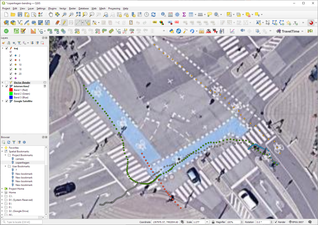
Let’s load the five test trajectories and the camera image to QGIS. To make sure that they align properly, both are set to the same CRS and I’ve created the following basic world file for the camera image:

1
0
0
-1
0
360

Then we can use the VectorBender tools to georeference the trajectories by linking locations from the camera image to locations on aerial images. You can see the whole process in action here:

After around 15 minutes linking control points, VectorBender comes up with the following georeferenced trajectory result:

Not bad for a quick-and-dirty hack. Some points on the borders of the image could not be georeferenced since I wasn’t always able to identify suitable control points at the camera image borders. So it won’t be perfect but should improve speed estimates.


This post is part of a series. Read more about movement data in GIS.

How to use Kaggle’s Taxi Trajectory Data in MovingPandas

Kaggle’s “Taxi Trajectory Data from ECML/PKDD 15: Taxi Trip Time Prediction (II) Competition” is one of the most used mobility / vehicle trajectory datasets in computer science. However, in contrast to other similar datasets, Kaggle’s taxi trajectories are provided in a format that is not readily usable in MovingPandas since the spatiotemporal information is provided as:

  • TIMESTAMP: (integer) Unix Timestamp (in seconds). It identifies the trip’s start;
  • POLYLINE: (String): It contains a list of GPS coordinates (i.e. WGS84 format) mapped as a string. The beginning and the end of the string are identified with brackets (i.e. [ and ], respectively). Each pair of coordinates is also identified by the same brackets as [LONGITUDE, LATITUDE]. This list contains one pair of coordinates for each 15 seconds of trip. The last list item corresponds to the trip’s destination while the first one represents its start;

Therefore, we need to create a DataFrame with one point + timestamp per row before we can use MovingPandas to create Trajectories and analyze them.

But first things first. Let’s download the dataset:

import datetime
import pandas as pd
import geopandas as gpd
import movingpandas as mpd
import opendatasets as od
from os.path import exists
from shapely.geometry import Point

input_file_path = 'taxi-trajectory/train.csv'

def get_porto_taxi_from_kaggle():
    if not exists(input_file_path):
        od.download("https://www.kaggle.com/datasets/crailtap/taxi-trajectory")

get_porto_taxi_from_kaggle()
df = pd.read_csv(input_file_path, nrows=10, usecols=['TRIP_ID', 'TAXI_ID', 'TIMESTAMP', 'MISSING_DATA', 'POLYLINE'])
df.POLYLINE = df.POLYLINE.apply(eval)  # string to list
df

And now for the remodelling:

def unixtime_to_datetime(unix_time):
    return datetime.datetime.fromtimestamp(unix_time)

def compute_datetime(row):
    unix_time = row['TIMESTAMP']
    offset = row['running_number'] * datetime.timedelta(seconds=15)
    return unixtime_to_datetime(unix_time) + offset

def create_point(xy):
    try: 
        return Point(xy)
    except TypeError:  # when there are nan values in the input data
        return None
 
new_df = df.explode('POLYLINE')
new_df['geometry'] = new_df['POLYLINE'].apply(create_point)
new_df['running_number'] = new_df.groupby('TRIP_ID').cumcount()
new_df['datetime'] = new_df.apply(compute_datetime, axis=1)
new_df.drop(columns=['POLYLINE', 'TIMESTAMP', 'running_number'], inplace=True)
new_df

And that’s it. Now we can create the trajectories:

trajs = mpd.TrajectoryCollection(
    gpd.GeoDataFrame(new_df, crs=4326), 
    traj_id_col='TRIP_ID', obj_id_col='TAXI_ID', t='datetime')
trajs.hvplot(title='Kaggle Taxi Trajectory Data', tiles='CartoLight')

That’s it. Now our MovingPandas.TrajectoryCollection is ready for further analysis.

By the way, the plot above illustrates a new feature in the recent MovingPandas 0.16 release which, among other features, introduced plots with arrow markers that show the movement direction. Other new features include a completely new custom distance, speed, and acceleration unit support. This means that, for example, instead of always getting speed in meters per second, you can now specify your desired output units, including km/h, mph, or nm/h (knots).


This post is part of a series. Read more about movement data in GIS.

MovingPandas v0.13 & v0.14 released!

December has been busy with two new MovingPandas releases: v0.13 and v0.14.

The latest v0.14 release is now available from conda-forge.

These releases are a huge step forward towards making MovingPandas easier to install with fewer mandatory dependencies. All interactive plotting libraries are now optional. So if you are using MovingPandas for trajectory data processing in the background and don’t need the interactive visualization features, the number of necessary libraries is now much lower. This (and the fact that GeoPandas is now shipped with OSGeo4W) will also make it easier to use MovingPandas in QGIS plugins.

New features:

  • #268 New add_angular_difference method

Includes fixes and enhancements for:

  • #267 Improved documentation: direction values are [0, 360)

Behind the scenes:

As always, all tutorials are available from the movingpandas-examples repository and on MyBinder:

If you have questions about using MovingPandas or just want to discuss new ideas, you’re welcome to join our discussion forum.

MovingPandas v0.12 released!

The latest v0.12 release is now available from conda-forge.

This release contains some really cool new features, including:

  • New function to add an acceleration column #253
  • We have further improved our repo setup by adding an action that automatically creates and publishes packages from releases, heavily inspired by the work of the GeoPandas team.
  • Last but not least, we’ve created a Twitter account for the project. (And might soon add a Mastodon account as well.)

As always, all tutorials are available from the movingpandas-examples repository and on MyBinder:

If you have questions about using MovingPandas or just want to discuss new ideas, you’re welcome to join our discussion forum.

MovingPandas v0.11 released!

The latest v0.11 release is now available from conda-forge.

This release contains some really cool new algorithms:

  • New minimum and Hausdorff distance measures #37
  • New functions to add a timedelta column and get the trajectory sampling interval #233 

As always, all tutorials are available from the movingpandas-examples repository and on MyBinder:

The new distance measures are covered in tutorial #11:

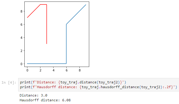
Computing distances between trajectories, as illustrated in tutorial #11

Computing distances between a trajectory and other geometry objects, as illustrated in tutorial #11

But don’t miss the great features covered by the other notebooks, such as outlier cleaning and smoothing:

Trajectory cleaning and smoothing, as illustrated in tutorial #10

If you have questions about using MovingPandas or just want to discuss new ideas, you’re welcome to join our discussion forum.

MovingPandas v0.10 released!

The latest v0.10 release is now available from conda-forge.

This release contains some really cool new algorithms:

If you have questions about using MovingPandas or just want to discuss new ideas, you’re welcome to join our recently opened discussion forum.

As always, all tutorials are available from the movingpandas-examples repository and on MyBinder:

Besides others examples, the movingpandas-examples repo contains the following tech demo: an interactive app built with Panel that demonstrates different MovingPandas stop detection parameters

To start the app, open the stopdetection-app.ipynb notebook and press the green Panel button in the Jupyter Lab toolbar:

MF-JSON update & tutorial with official sample

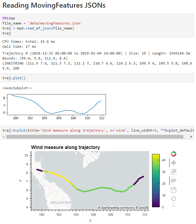
Since last week’s post, I’ve learned that there is an official OGC Moving Features JSON Encodings repository with more recent sample datasets, including MovingPoint, MovingPolygon, and Trajectory JSON examples.

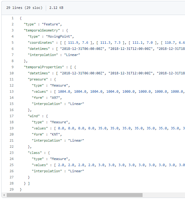
The MovingPoint example seems to describe a storm, including its path (temporalGeometry), pressure, wind strength, and class values (temporalProperties):

You can give the current implementation a spin using this MyBinder notebook

An exciting future step would be to experiment with extending MovingPandas to support the MovingPolygon MF-JSON examples. MovingPolygons can change their size and orientation as they move. I’m not yet sure, however, if the number of polygon nodes can change between time steps and how this would be reflected by the prism concept presented in the draft specification:

Image source: https://ksookim.github.io/mf-json/

New OGC Moving Features JSON support in MovingPandas

First time, we talked about the OGC Moving Features standard in a post from 2017. Back then, we looked at the proposed standard way to encode trajectories in CSV and discussed its issues. Since then, the Moving Features working group at OGC has not been idle. Besides the CSV and XML encodings, they have designed a new JSON encoding that addresses many of the downsides of the previous two. You can read more about this in our 2020 preprint “From Simple Features to Moving Features and Beyond”.

Basically Moving Features JSON (MF-JSON) is heavily inspired by GeoJSON and it comes with a bunch of mandatory and optional key/value pairs. There is support for static properties as well as dynamic temporal properties and, of course, temporal geometries (yes geometries, not just points).

I think this format may have an actual chance of gaining more widespread adoption.

Image source: http://www.opengis.net/doc/BP/mf-json/1.0

Inspired by Pandas.read_csv() and GeoPandas.read_file(), I’ve started implementing a read_mf_json() function in MovingPandas. So far, it supports basic MovingFeature JSONs with MovingPoint geometry:

You’ll need to use the current development version to test this feature.

Next steps will be MovingFeatureCollection JSONs and support for static as well as temporal properties. We’ll have to see if MovingPandas can be extended to go beyond moving point geometries. Storing moving linestrings and polygons in the GeoDataFrame will be the simple part but analytics and visualization will certainly be more tricky.


This post is part of a series. Read more about movement data in GIS.

Geospatial: where MovingPandas meets Leafmap

Many of you certainly have already heard of and/or even used Leafmap by Qiusheng Wu.

Leafmap is a Python package for interactive spatial analysis with minimal coding in Jupyter environments. It provides interactive maps based on folium and ipyleaflet, spatial analysis functions using WhiteboxTools and whiteboxgui, and additional GUI elements based on ipywidgets.

This way, Leafmap achieves a look and feel that is reminiscent of a desktop GIS:

Image source: https://github.com/giswqs/leafmap

Recently, Qiusheng has started an additional project: the geospatial meta package which brings together a variety of different Python packages for geospatial analysis. As such, the main goals of geospatial are to make it easier to discover and use the diverse packages that make up the spatial Python ecosystem.

Besides the usual suspects, such as GeoPandas and of course Leafmap, one of the packages included in geospatial is MovingPandas. Thanks, Qiusheng!

I’ve tested the mamba install today and am very happy with how this worked out. There is just one small hiccup currently, which is related to an upstream jinja2 issue. After installing geospatial, I therefore downgraded jinja:

mamba install -c conda-forge geospatial 
mamba install -c conda-forge jinja2=3.0

Of course, I had to try Leafmap and MovingPandas in action together. Therefore, I fired up one of the MovingPandas example notebook (here the example on clipping trajectories using polygons). As you can see, the integration is pretty smooth since Leafmap already support drawing GeoPandas GeoDataFrames and MovingPandas can convert trajectories to GeoDataFrames (both lines and points):

Clipped trajectory segments as linestrings in Leafmap
Leafmap includes an attribute table view that can be activated on user request to show, e.g. trajectory information
And, of course, we can also map the original trajectory points

Geospatial also includes the new dask-geopandas library which I’m very much looking forward to trying out next.

MovingPandas now supports local coordinates

MovingPandas 0.9rc3 has just been released, including important fixes for local coordinate support. Sports analytics is just one example of movement data analysis that uses local rather than geographic coordinates.

Many movement data sources – such as soccer players’ movements extracted from video footage – use local reference systems. This means that x and y represent positions within an arbitrary frame, such as a soccer field.

Since Geopandas and GeoViews support handling and plotting local coordinates just fine, there is nothing stopping us from applying all MovingPandas functionality to this data. For example, to visualize the movement speed of players:

Of course, we can also plot other trajectory attributes, such as the team affiliation.

But one particularly useful feature is the ability to use custom background images, for example, to show the soccer field layout:

To access the full example notebook, visit: https://github.com/anitagraser/movingpandas/blob/master/tutorials/5-local-coordinates.ipynb

An update to the MovingPandas examples repository will follow shortly.

MovingPandas v0.9 released!

The latest v0.9 release is now available from conda-forge.

This release contains some really cool new algorithms:

The Kalman filter in action on the Geolife sample: smoother, less jiggly trajectories.
Top-Down Time Ratio generalization aka trajectory compression in action: reduces the number of positions along the trajectory without altering the spatiotemporal properties, such as speed, too much.

These new algorithms were contributed by Lyudmil Vladimirov and George S. Theodoropoulos.

Behind the scenes, Ray Bell took care of moving testing from Travis to Github Actions, and together we worked through the steps to ensure that the source code is now properly linted using flake8 and black.

Being able to work with so many awesome contributors has made this release really special for me. It’s great to see the project attracting more developer interest.

As always, all tutorials are available from the movingpandas-examples repository and on MyBinder:

MovingPandas v0.8 released!

The latest v0.8 release is now available from conda-forge.

New features include:

  • More convenient creation of TrajectoryCollection objects from (Geo)DataFrames (#137)
  • Support for different geometry column names (#112)

Last week, I also had the pleasure to speak about MovingPandas at Carto’s Spatial Data Science Conference SDSC21:

As always, all tutorials are available from the movingpandas-examples repository and on MyBinder:

MovingPandas v0.7 released!

The latest v0.7 release is now available from conda-forge.

New features include:

As always, all tutorials are available from the movingpandas-examples repository and on MyBinder:

Movement data in GIS #35: stop detection & analysis with MovingPandas

In the last few days, there’s been a sharp rise in interest in vessel movements, and particularly, in understanding where and why vessels stop. Following the grounding of Ever Given in the Suez Canal, satellite images and vessel tracking data (AIS) visualizations are everywhere:

Using movement data analytics tools, such as MovingPandas, we can dig deeper and explore patterns in the data.

The MovingPandas.TrajectoryStopDetector is particularly useful in this situation. We can provide it with a Trajectory or TrajectoryCollection and let it detect all stops, that is, instances were the moving object stayed within a certain area (with a diameter of 1000m in this example) for a an extended duration (at least 3 hours).

stops = mpd.TrajectoryStopDetector(trajs).get_stop_segments(
    min_duration=timedelta(hours=3), max_diameter=1000)

The resulting stop segments include spatial and temporal information about the stop location and duration. To make this info more easily accessible, let’s turn the stop segment TrajectoryCollection into a point GeoDataFrame:

stop_pts = gpd.GeoDataFrame(columns=['geometry']).set_geometry('geometry')
stop_pts['stop_id'] = [track.id for track in stops.trajectories]
stop_pts= stop_pts.set_index('stop_id')

for stop in stops:
    stop_pts.at[stop.id, 'ID'] = stop.df['ID'][0]
    stop_pts.at[stop.id, 'datetime'] = stop.get_start_time()
    stop_pts.at[stop.id, 'duration_h'] = stop.get_duration().total_seconds()/3600
    stop_pts.at[stop.id, 'geometry'] = stop.get_start_location()

Indeed, I think the next version of MovingPandas should include a function that directly returns stops as points.

Now we can explore the stop information. For example, the map plot shows that stops are concentrated in three main areas: the northern and southern ends of the Canal, as well as the Great Bitter Lake in the middle. By looking at the timing of stops and their duration in a scatter plot, we can clearly see that the Ever Given stop (red) caused a chain reaction: the numerous points lining up on the diagonal of the scatter plot represent stops that very likely are results of the blockage:

Before the grounding, the stop distribution nicely illustrates the canal schedule. Vessels have to wait until it’s turn for their direction to go through:

You can see the full analysis workflow in the following video. Please turn on the captions for details.

Huge thanks to VesselsValue for supplying the data!

For another example of MovingPandas‘ stop dectection in action, have a look at Bryan R. Vallejo’s tutorial on detecting stops in bird tracking data which includes some awesome visualizations using KeplerGL:

Kepler.GL visualization by Bryan R. Vallejo

This post is part of a series. Read more about movement data in GIS.

Movement data in GIS #34: a protocol for exploring movement data

After writing “Towards a template for exploring movement data” last year, I spent a lot of time thinking about how to develop a solid approach for movement data exploration that would help analysts and scientists to better understand their datasets. Finally, my search led me to the excellent paper “A protocol for data exploration to avoid common statistical problems” by Zuur et al. (2010). What they had done for the analysis of common ecological datasets was very close to what I was trying to achieve for movement data. I followed Zuur et al.’s approach of a exploratory data analysis (EDA) protocol and combined it with a typology of movement data quality problems building on Andrienko et al. (2016). Finally, I brought it all together in a Jupyter notebook implementation which you can now find on Github.

There are two options for running the notebook:

  1. The repo contains a Dockerfile you can use to spin up a container including all necessary datasets and a fitting Python environment.
  2. Alternatively, you can download the datasets manually and set up the Python environment using the provided environment.yml file.

The dataset contains over 10 million location records. Most visualizations are based on Holoviz Datashader with a sprinkling of MovingPandas for visualizing individual trajectories.

Point density map of 10 million location records, visualized using Datashader

Line density map for detecting gaps in tracks, visualized using Datashader

Example trajectory with strong jitter, visualized using MovingPandas & GeoViews


I hope this reference implementation will provide a starting point for many others who are working with movement data and who want to structure their data exploration workflow.

If you want to dive deeper, here’s the paper:

[1] Graser, A. (2021). An exploratory data analysis protocol for identifying problems in continuous movement data. Journal of Location Based Services. doi:10.1080/17489725.2021.1900612.
(If you don’t have institutional access to the journal, the publisher provides 50 free copies using this link. Once those are used up, just leave a comment below and I can email you a copy.)

References


This post is part of a series. Read more about movement data in GIS.
MovingPandas v0.5 released!

The latest v0.5 release is now available from conda-forge.

New features include:

As always, all tutorials are available on MyBinder:


Detected stops (left) and trajectory split at stops (right)

Super-quick interactive data & parameter exploration

This post introduces Holoviz Panel, a library that makes it possible to create really quick dashboards in notebook environments as well as more sophisticated custom interactive web apps and dashboards.

The following example shows how to use Panel to explore a dataset (a trajectory collection in this case) and different parameter settings (relating to trajectory generalization). All the Panel code we need is a dict that defines the parameters that we want to explore. Then we can use Panel’s interact function to automatically generate a dashboard for our custom plotting function:

import panel as pn

kw = dict(traj_id=(1, len(traj_collection)), 
          tolerance=(10, 100, 10), 
          generalizer=['douglas-peucker', 'min-distance'])
pn.interact(plot_generalized, **kw)

Click to view the resulting dashboard in full resolution:

The plotting function uses the parameters to generate a Holoviews plot. First it fetches a specific trajectory from the trajectory collection. Then it generalizes the trajectory using the specified parameter settings. As you can see, we can easily combine maps and other plots to visualize different aspects of the data:

def plot_generalized(traj_id=1, tolerance=10, generalizer='douglas-peucker'):
  my_traj = traj_collection.get_trajectory(traj_id).to_crs(CRS(4088))
  if generalizer=='douglas-peucker':
    generalized = mpd.DouglasPeuckerGeneralizer(my_traj).generalize(tolerance)
  else:
    generalized = mpd.MinDistanceGeneralizer(my_traj).generalize(tolerance)
  generalized.add_speed(overwrite=True)
  return ( 
    generalized.hvplot(
      title='Trajectory {} (tolerance={})'.format(my_traj.id, tolerance), 
      c='speed', cmap='Viridis', colorbar=True, clim=(0,20), 
      line_width=10, width=500, height=500) + 
    generalized.df['speed'].hvplot.hist(
      title='Speed histogram', width=300, height=500) 
    )

Trajectory collections and generalization functions used in this example are part of the MovingPandas library. If you are interested in movement data analysis, you should check it out! You can find this example notebook in the MovingPandas tutorial section.

MovingPandas v0.3 released!

MovingPandas has come a long way since 2018 when I started to experiment with GeoPandas for trajectory data handling.

This week, MovingPandas passed peer review and was approved for pyOpenSci. This technical review process was extremely helpful in ensuring code, project, and documentation quality. I would strongly recommend it to everyone working on new data science libraries!

The lastest v0.3 release is now available from conda-forge.

All tutorials are available on MyBinder

New features include:

  • Support for GeoPandas 0.7
  • Trajectory collection aggregation functions to generate flow maps


Movement data in GIS #29: power your web apps with movement data using mobilitydb-sqlalchemy

This is a guest post by Bommakanti Krishna Chaitanya @chaitan94

Introduction

This post introduces mobilitydb-sqlalchemy, a tool I’m developing to make it easier for developers to use movement data in web applications. Many web developers use Object Relational Mappers such as SQLAlchemy to read/write Python objects from/to a database.

Mobilitydb-sqlalchemy integrates the moving objects database MobilityDB into SQLAlchemy and Flask. This is an important step towards dealing with trajectory data using appropriate spatiotemporal data structures rather than plain spatial points or polylines.

To make it even better, mobilitydb-sqlalchemy also supports MovingPandas. This makes it possible to write MovingPandas trajectory objects directly to MobilityDB.

For this post, I have made a demo application which you can find live at https://mobilitydb-sqlalchemy-demo.adonmo.com/. The code for this demo app is open source and available on GitHub. Feel free to explore both the demo app and code!

In the following sections, I will explain the most important parts of this demo app, to show how to use mobilitydb-sqlalchemy in your own webapp. If you want to reproduce this demo, you can clone the demo repository and do a “docker-compose up –build” as it automatically sets up this docker image for you along with running the backend and frontend. Just follow the instructions in README.md for more details.

Declaring your models

For the demo, we used a very simple table – with just two columns – an id and a tgeompoint column for the trip data. Using mobilitydb-sqlalchemy this is as simple as defining any regular table:

from flask_sqlalchemy import SQLAlchemy
from mobilitydb_sqlalchemy import TGeomPoint

db = SQLAlchemy()

class Trips(db.Model):
   __tablename__ = "trips"
   trip_id = db.Column(db.Integer, primary_key=True)
   trip = db.Column(TGeomPoint)

Note: The library also allows you to use the Trajectory class from MovingPandas as well. More about this is explained later in this tutorial.

Populating data

When adding data to the table, mobilitydb-sqlalchemy expects data in the tgeompoint column to be a time indexed pandas dataframe, with two columns – one for the spatial data  called “geometry” with Shapely Point objects and one for the temporal data “t” as regular python datetime objects.

from datetime import datetime
from shapely.geometry import Point

# Prepare and insert the data
# Typically it won’t be hardcoded like this, but it might be coming from 
# other data sources like a different database or maybe csv files
df = pd.DataFrame(
   [
       {"geometry": Point(0, 0), "t": datetime(2012, 1, 1, 8, 0, 0),},
       {"geometry": Point(2, 0), "t": datetime(2012, 1, 1, 8, 10, 0),},
       {"geometry": Point(2, -1.9), "t": datetime(2012, 1, 1, 8, 15, 0),},
   ]
).set_index("t")

trip = Trips(trip_id=1, trip=df)
db.session.add(trip)
db.session.commit()

Writing queries

In the demo, you see two modes. Both modes were designed specifically to explain how functions defined within MobilityDB can be leveraged by our webapp.

1. All trips mode – In this mode, we extract all trip data, along with distance travelled within each trip, and the average speed in that trip, both computed by MobilityDB itself using the ‘length’, ‘speed’ and ‘twAvg’ functions. This example also shows that MobilityDB functions can be chained to form more complicated queries.

mobilitydb-sqlalchemy-demo-1

trips = db.session.query(
   Trips.trip_id,
   Trips.trip,
   func.length(Trips.trip),
   func.twAvg(func.speed(Trips.trip))
).all()

2. Spatial query mode – In this mode, we extract only selective trip data, filtered by a user-selected region of interest. We then make a query to MobilityDB to extract only the trips which pass through the specified region. We use MobilityDB’s ‘intersects’ function to achieve this filtering at the database level itself.

mobilitydb-sqlalchemy-demo-2

trips = db.session.query(
   Trips.trip_id,
   Trips.trip,
   func.length(Trips.trip),
   func.twAvg(func.speed(Trips.trip))
).filter(
   func.intersects(Point(lat, lng).buffer(0.01).wkb, Trips.trip),
).all()

Using MovingPandas Trajectory objects

Mobilitydb-sqlalchemy also provides first-class support for MovingPandas Trajectory objects, which can be installed as an optional dependency of this library. Using this Trajectory class instead of plain DataFrames allows us to make use of much richer functionality over trajectory data like analysis speed, interpolation, splitting and simplification of trajectory points, calculating bounding boxes, etc. To make use of this feature, you have set the use_movingpandas flag to True while declaring your model, as shown in the below code snippet.

class TripsWithMovingPandas(db.Model):
   __tablename__ = "trips"
   trip_id = db.Column(db.Integer, primary_key=True)
   trip = db.Column(TGeomPoint(use_movingpandas=True))

Now when you query over this table, you automatically get the data parsed into Trajectory objects without having to do anything else. This also works during insertion of data – you can directly assign your movingpandas Trajectory objects to the trip column. In the below code snippet we show how inserting and querying works with movingpandas mode.

from datetime import datetime
from shapely.geometry import Point

# Prepare and insert the data
# Typically it won’t be hardcoded like this, but it might be coming from 
# other data sources like a different database or maybe csv files
df = pd.DataFrame(
   [
       {"geometry": Point(0, 0), "t": datetime(2012, 1, 1, 8, 0, 0),},
       {"geometry": Point(2, 0), "t": datetime(2012, 1, 1, 8, 10, 0),},
       {"geometry": Point(2, -1.9), "t": datetime(2012, 1, 1, 8, 15, 0),},
   ]
).set_index("t")

geo_df = GeoDataFrame(df)
traj = mpd.Trajectory(geo_df, 1)

trip = Trips(trip_id=1, trip=traj)
db.session.add(trip)
db.session.commit()

# Querying over this table would automatically map the resulting tgeompoint 
# column to movingpandas’ Trajectory class
result = db.session.query(TripsWithMovingPandas).filter(
   TripsWithMovingPandas.trip_id == 1
).first()

print(result.trip.__class__)
# <class 'movingpandas.trajectory.Trajectory'>

Bonus: trajectory data serialization

Along with mobilitydb-sqlalchemy, recently I have also released trajectory data serialization/compression libraries based on Google’s Encoded Polyline Format Algorithm, for python and javascript called trajectory and trajectory.js respectively. These libraries let you send trajectory data in a compressed format, resulting in smaller payloads if sending your data through human-readable serialization formats like JSON. In some of the internal APIs we use at Adonmo, we have seen this reduce our response sizes by more than half (>50%) sometimes upto 90%.

Want to learn more about mobilitydb-sqlalchemy? Check out the quick start & documentation.


This post is part of a series. Read more about movement data in GIS.

First working MovingPandas setup on Databricks

In December, I wrote about GeoPandas on Databricks. Back then, I also tried to get MovingPandas working but without luck. (While GeoPandas can be installed using Databricks’ dbutils.library.installPyPI("geopandas") this PyPI install just didn’t want to work for MovingPandas.)

Now that MovingPandas is available from conda-forge, I gave it another try and … *spoiler alert* … it works!

First of all, conda support on Databricks is in beta. It’s not included in the default runtimes. At the time of writing this post, “6.0 Conda Beta” is the latest runtime with conda:

Once the cluster is up and connected to the notebook, a quick conda list shows the installed packages:

Time to install MovingPandas! I went with a 100% conda-forge installation. This takes a looong time (almost half an hour)!

When the installs are finally done, it get’s serious: time to test the imports!

Success!

Now we can put the MovingPandas data structures to good use. But first we need to load some movement data:

Or course, the points in this GeoDataFrame can be plotted. However, the plot isn’t automatically displayed once plot() is called on the GeoDataFrame. Instead, Databricks provides a display() function to display Matplotlib figures:

MovingPandas also uses Matplotlib. Therefore we can use the same approach to plot the TrajectoryCollection that can be created from the GeoDataFrame:

These Matplotlib plots are nice and quick but they lack interactivity and therefore are of limited use for data exploration.

MovingPandas provides interactive plotting (including base maps) using hvplot. hvplot is based on Bokeh and, luckily, the Databricks documentation tells us that bokeh plots can be exported to html and then displayed using  displayHTML():

Of course, we could achieve all this on MyBinder as well (and much more quickly). However, Databricks gets interesting once we can add (Py)Spark and distributed processing to the mix. For example, “Getting started with PySpark & GeoPandas on Databricks” shows a spatial join function that adds polygon information to a point GeoDataFrame.

A potential use case for MovingPandas would be to speed up flow map computations. The recently added aggregator functionality (currently in master only) first computes clusters of significant trajectory points and then aggregates the trajectories into flows between these clusters. Matching trajectory points to the closest cluster could be a potential use case for distributed computing. Each trajectory (or each point) can be handled independently, only the cluster locations have to be broadcast to all workers.

Flow map (screenshot from MovingPandas tutorial 4_generalization_and_aggregation.ipynb)


  • Page 1 of 2 ( 22 posts )
  • >>
  • movingpandas

Back to Top

Sustaining Members