Related Plugins and Tags

QGIS Planet

Movement data in GIS #3: visualizing massive trajectory datasets

In the fist two parts of the Movement Data in GIS series, I discussed modeling trajectories as LinestringM features in PostGIS to overcome some common issues of movement data in GIS and presented a way to efficiently render speed changes along a trajectory in QGIS without having to split the trajectory into shorter segments.

While visualizing individual trajectories is important, the real challenge is trying to visualize massive trajectory datasets in a way that enables further analysis. The out-of-the-box functionality of GIS is painfully limited. Except for some transparency and heatmap approaches, there is not much that can be done to help interpret “hairballs” of trajectories. Luckily researchers in visual analytics have already put considerable effort into finding solutions for this visualization challenge. The approach I want to talk about today is by Andrienko, N., & Andrienko, G. (2011). Spatial generalization and aggregation of massive movement data. IEEE Transactions on visualization and computer graphics, 17(2), 205-219. and consists of the following main steps:

  1. Extracting characteristic points from the trajectories
  2. Grouping the extracted points by spatial proximity
  3. Computing group centroids and corresponding Voronoi cells
  4. Deviding trajectories into segments according to the Voronoi cells
  5. Counting transitions from one cell to another

The authors do a great job at describing the concepts and algorithms, which made it relatively straightforward to implement them in QGIS Processing. So far, I’ve implemented the basic logic but the paper contains further suggestions for improvements. This was also my first pyQGIS project that makes use of the measurement value support in the new geometry engine. The time information stored in the m-values is used to detect stop points, which – together with start, end, and turning points – make up the characteristic points of a trajectory.

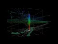
The following animation illustrates the current state of the implementation: First the “hairball” of trajectories is rendered. Then we extract the characteristic points and group them by proximity. The big black dots are the resulting group centroids. From there, I skipped the Voronoi cells and directly counted transitions from “nearest to centroid A” to “nearest to centroid B”.

(data credits: GeoLife project)

From thousands of individual trajectories to a generalized representation of overall movement patterns (data credits: GeoLife project, map tiles: Stamen, map data: OSM)

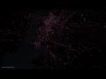
The resulting visualization makes it possible to analyze flow strength as well as directionality. I have deliberately excluded all connections with a count below 10 transitions to reduce visual clutter. The cell size / distance between point groups – and therefore the level-of-detail – is one of the input parameters. In my example, I used a target cell size of approximately 2km. This setting results in connections which follow the major roads outside the city center very well. In the city center, where the road grid is tighter, trajectories on different roads mix and the connections are less clear.

Since trajectories in this dataset are not limited to car trips, it is expected to find additional movement that is not restricted to the road network. This is particularly noticeable in the dense area in the west where many slow trajectories – most likely from walking trips – are located. The paper also covers how to ensure that connections are limited to neighboring cells by densifying the trajectories before computing step 4.

trajectory_generalization

Running the scripts for over 18,000 trajectories requires patience. It would be worth evaluating if the first three steps can be run with only a subsample of the data without impacting the results in a negative way.

One thing I’m not satisfied with yet is the way to specify the target cell size. While it’s possible to measure ellipsoidal distances in meters using QgsDistanceArea (irrespective of the trajectory layer’s CRS), the initial regular grid used in step 2 in order to group the extracted points has to be specified in the trajectory layer’s CRS units – quite likely degrees. Instead, it may be best to transform everything into an equidistant projection before running any calculations.

It’s good to see that PyQGIS enables us to use the information encoded in PostGIS LinestringM features to perform spatio-temporal analysis. However, working with m or z values involves a lot of v2 geometry classes which work slightly differently than their v1 counterparts. It certainly takes some getting used to. This situation might get cleaned up as part of the QGIS 3 API refactoring effort. If you can, please support work on QGIS 3. Now is the time to shape the PyQGIS API for the following years!


What went on at FOSS4G 2015?

Granted, I could only follow FOSS4G 2015 remotely on social media but what I saw was quite impressive and will keep me busy exploring for quite a while. Here’s my personal pick of this year’s highlights which I’d like to share with you:

QGIS

Marco Hugentobler at FOSS4G 2015 (Photo by Jody Garnett)

Marco Hugentobler at FOSS4G 2015 (Photo by Jody Garnett)

The Sourcepole team has been particularly busy with four presentations which you can find on their blog.

Marco Hugentobler’s keynote is just great, summing up the history of the QGIS project and discussing success factor for open source projects.

Marco also gave a second presentation on new QGIS features for power users, including live layer effects, new geometry support (curves!), and geometry checker.

There has also been an update to QTiles plugin by NextGIS this week.

If you’re a bit more into webmapping, Victor Olaya presented the Web App Builder he’s been developing at Boundless. Web App Builder should appear in the official plugin repo soon.

Preview of Web App Builder from Victors presentation

Preview of Web App Builder from Victors presentation

Geocoding

If you work with messy, real-world data, you’ve most certainly been fighting with geocoding services, trying to make the best of a bunch of address lists. The Python Geocoder library promises to make dealing with geocoding services such as Google, Bing, OSM & many easier than ever before.

Let me know if you tried it.

Mobmap Visualizations

Mobmap – or more specifically Mobmap2 – is an extension for Chrome which offers visualization and analysis capabilities for trajectory data. I haven’t tried it yet but their presentation certainly looks very interesting:


Trajectory animations with fadeout effect

Today’s post is a short tutorial for creating trajectory animations with a fadeout effect using QGIS Time Manager. This is the result we are aiming for:

The animation shows the current movement in pink which fades out and leaves behind green traces of the trajectories.

About the data

GeoLife GPS Trajectories were collected within the (Microsoft Research Asia) Geolife project by 182 users in a period of over three years (from April 2007 to August 2012). [1,2,3] The GeoLife GPS Trajectories download contains many text files organized in multiple directories. The data files are basically CSVs with 6 lines of header information. They contain the following fields:

Field 1: Latitude in decimal degrees.
Field 2: Longitude in decimal degrees.
Field 3: All set to 0 for this dataset.
Field 4: Altitude in feet (-777 if not valid).
Field 5: Date – number of days (with fractional part) that have passed since 12/30/1899.
Field 6: Date as a string.
Field 7: Time as a string.

Data prep: PostGIS

Since any kind of GIS operation on text files will be quite inefficient, I decided to load the data into a PostGIS database. This table of millions of GPS points can then be sliced into appropriate chunks for exploration, for example, a day in Beijing:

CREATE MATERIALIZED VIEW geolife.beijing 
AS SELECT trajectories.id,
    trajectories.t_datetime,
    trajectories.t_datetime + interval '1 day' as t_to_datetime,
    trajectories.geom,
    trajectories.oid
   FROM geolife.trajectories
   WHERE st_dwithin(trajectories.geom,
           st_setsrid(
             st_makepoint(116.3974589, 
                           39.9388838), 
             4326), 
           0.1) 
   AND trajectories.t_datetime >= '2008-11-11 00:00:00'
   AND trajectories.t_datetime < '2008-11-12 00:00:00'
WITH DATA

Trajectory viz: a fadeout effect for point markers

The idea behind this visualization is to show both the current movement as well as the history of the trajectories. This can be achieved with a fadeout effect which leaves behind traces of past movement while the most recent positions are highlighted to stand out.

Map tiles by Stamen Design, under CC BY 3.0. Data by OpenStreetMap, under ODbL.

Map tiles by Stamen Design, under CC BY 3.0. Data by OpenStreetMap, under ODbL.

This effect can be created using a Single Symbol renderer with a marker symbol with two symbol layers: one layer serves as the highlights layer (pink) while the second layer represents the traces (green) which linger after the highlights disappear. Feature blending is used to achieve the desired effect for overlapping markers.

Screenshot 2015-05-06 23.52.40

The highlights layer has two expression-based properties: color and size. The color fades to white and the point size shrinks as the point ages. The age can be computed by comparing the point’s t_datetime timestamp to the Time Manager animation time $animation_datetime.

This expression creates the color fading effect:

color_hsv(  
  311,
  scale_exp( 
    minute(age($animation_datetime,"t_datetime")),
    0,60,
    100,0,
    0.2
  ),
  90
)

and this expression makes the point size shrink:

scale_exp( 
  minute(age($animation_datetime,"t_datetime")),
  0,60,
  24,0,
  0.2
)

Outlook

I’m currently preparing this and a couple of other examples for my Time Manager workshop at the upcoming 1st QGIS conference in Nødebo. The workshop materials will be made available online afterwards.

Literature

[1] Yu Zheng, Lizhu Zhang, Xing Xie, Wei-Ying Ma. Mining interesting locations and travel sequences from GPS trajectories. In Proceedings of International conference on World Wild Web (WWW 2009), Madrid Spain. ACM Press: 791-800.
[2] Yu Zheng, Quannan Li, Yukun Chen, Xing Xie, Wei-Ying Ma. Understanding Mobility Based on GPS Data. In Proceedings of ACM conference on Ubiquitous Computing (UbiComp 2008), Seoul, Korea. ACM Press: 312-321.
[3] Yu Zheng, Xing Xie, Wei-Ying Ma, GeoLife: A Collaborative Social Networking Service among User, location and trajectory. Invited paper, in IEEE Data Engineering Bulletin. 33, 2, 2010, pp. 32-40.


Dataviz with OpenSource Tools

Today, I’ve finished my submission for the Hubway Data Visualization Challenge. All parts of the resulting dataviz were created using open source tools. My toolbox for this work contains: QGIS, Spatialite, Inkscape, Gimp and Open Office Calc. To see the complete submission and read more about it, check the project page.


Exploring Hubway’s Data II

Today, I’ve been experimenting with a new way to visualize origin-destination pairs (ODs). The following image shows my first results:

The ideas was to add a notion of direction as well as uncertainty. The “flower petals” have a pointed origin and grow wider towards the middle. (Looking at the final result, they should probably go much narrower towards the end again.) The area covered by the petals is a simple approximation of where I’d expect the bike routes without performing any routing.

To get there, I reprojected the connection lines to EPSG:3857 and calculated connection length and line orientation using QGIS Field Calculator $length operator and the bearing formula given in QGIS Wiki:

(atan((xat(-1)-xat(0))/(yat(-1)-yat(0)))) * 180/3.14159 + (180 *(((yat(-1)-yat(0)) < 0) + (((xat(-1)-xat(0)) < 0 AND (yat(-1) - yat(0)) >0)*2)))

For the style, I created a new “flower petal” SVG symbol in Inkscape and styled it with varying transparency values: Rare connections are more transparent than popular ones. This style is applied to the connection start points. Using the advanced options “size scale” and “rotation”, it is possible to rotate the petals into the right direction as well as scale them using the previously calculated values for connection length and orientation.

Update

While the above example uses pretty wide petals this one is done with a much narrower petal. I think it’s more appropriate for the data at hand:

Most of the connections are clearly heading south east, across Charles River, except for that group of connections pointing the opposite direction, to Harvard Square.


Exploring Hubway’s Data I

Hubway is a bike sharing system in Boston and they are currently hosting a data visualization challenge. What a great chance to play with some real-world data!

To get started, I loaded both station Shapefile and trip CSV into a new Spatialite database. The GUI is really helpful here – everything is done in a few clicks. Afterwards, I decided to look into which station combinations are most popular. The following SQL script creates my connections table:

create table connections (
start_station_id INTEGER,
end_station_id INTEGER,
count INTEGER,
Geometry GEOMETRY);


insert into connections select 
start_station_id, 
end_station_id, 
count(*) as count, 
LineFromText('LINESTRING('||X(a.Geometry)||' '||Y(a.Geometry)||','
                          ||X(b.Geometry)||' '||Y(b.Geometry)||')') as Geometry
 from trips, stations a, stations b
where start_station_id = a.ID 
and end_station_id = b.ID
and a.ID != b.ID
and a.ID is not NULL
and b.ID is not NULL
group by start_station_id, end_station_id;

(Note: This is for Spatialite 2.4, so there is no MakeLine() method. Use MakeLine if you are using 3.0.)

For a first impression, I decided to map popular connections with more than one hundred entries. Wider lines mean more entries. The points show the station locations and they are color coded by starting letter. (I’m not yet sure if they mean anything. They seem to form groups.)

Some of the stations don’t seem to have any strong connections at all. Others are rather busy. The city center and the dark blue axis pointing west seem most popular.

I’m really looking forward to what everyone else will be finding in this dataset.


Exploring Mobility Data Using Time Manager

Data from various vehicles is collected for many purposes in cities worldwide. To get a feeling for just how much data is available, I created the following video using QGIS Time Manager which has been shown at the Austrian Museum of Applied Arts “MADE 4 YOU – Design for Change”. It shows one hour of taxi tracks in the city of Vienna:

If you like the video, please go to http://www.ertico.com/2012-its-video-competition-open-vote and vote for it in the category “Videos directed at the general public”.


Space-Time Cubes – Exploring Twitter Streams III

This post continues my quest of exploring the spatial dimension of Twitter streams. I wanted to try one of the classic spatio-temporal visualization methods: Space-time cubes where the vertical axis represents time while the other two map space. Like the two previous examples, this visualization is written in pyprocessing, a Python port of the popular processing environment.

This space-time cube shows twitter trajectories that contain at least one tweet in New York Times Square. The 24-hour day starts at the bottom of the cube and continues to the top. Trajectories are colored based on the time stamp of their start tweet.

Additionally, all trajectories are also drawn in context of the coastline (data: OpenStreetMap) on the bottom of the cube.

While there doesn’t seem to be much going on in the early morning hours, we can see quite a busy coming and going during the afternoon and evening. From the bunch of vertical lines over Times Square, we can also assume that some of our tweet authors spent a considerable time at and near Times Square.

I’ve also created an animated version. Again, I recommend to watch it in HD.


A Visual Exploration of Twitter Streams II

After my first shot at analyzing Twitter data visually I received a lot of great feedback. Thank you!

For my new attempt, I worked on incorporating your feedback such as: filter unrealistic location changes, show connections “grow” instead of just popping up and zoom to an interesting location. The new animation therefore focuses on Manhattan – one of the places with reasonably high geotweet coverage.

The background is based on OpenStreetMap coastline data which I downloaded using QGIS OSM plugin and rendered in pyprocessing together with the geotweets. To really see what’s going on, switch to HD resolution and full screen:

It’s pretty much work-in-progress. The animation shows similar chaotic patterns seen in other’s attempts at animating tweets. To me, the distribution of tweets looks reasonable and many of the connection lines seem to actually coincide with the bridges spanning to and from Manhattan.

This work is an attempt at discovering the potential of Twitter data and at the same time learning some pyprocessing which will certainly be useful for many future tasks. The next logical step seems to be to add information about interactions between users and/or to look at the message content. Another interesting task would be to add interactivity to the visualization.


A Visual Exploration of Twitter Streams

Twitter streams are curious things, especially the spatial data part. I’ve been using Tweepy to collect tweets from the public timeline and what did I discover? Tweets can have up to three different spatial references: “coordinates”, “geo” and “place”. I’ll still have to do some more reading on how to interpret these different attributes.

For now, I have been using “coordinates” to explore the contents of a stream which was collected over a period of five hours using

stream.filter(follow=None,locations=(-180,-90,180,90))

for global coverage. In the video, each georeferenced tweet produces a new dot on the map and if the user’s coordinates change, a blue arrow is drawn:

While pretty, these long blue arrows seem rather suspicious. I’ve only been monitoring the stream for around five hours. Any cross-Atlantic would take longer than that. I’m either misinterpreting the tweets or these coordinates are fake. Seems like it is time to dive deeper into the data.


  • Page 1 of 1 ( 10 posts )
  • dataviz

Back to Top

Sustaining Members