Sorry, this entry is only available in French.

The PostgreSQL Connection Service File pg_service.conf is nothing new. It has existed for quite some time and maybe you have already used it sometimes too. But not only the new QGIS plugin PG service parser is a reason to write about our love for this file, as well we generally think it’s time to show you how it can be used for really cool things.

What is the Connection Service File?

The Connection Service File allows you to save connection settings for each so-called “service” locally.

So when you have a database called gis on a local PostgreSQL with port 5432 and username/password is docker/docker you can store this as a service called my-local-gis.

# Local GIS Database for Testing purposes

host=localhost port=5432 dbname=gis user=docker password=docker

This Connection Service File is called pg_service.conf and is by client applications (such as psql or QGIS) generally found directly in the user directory. In Windows it is then found in the user’s application directory postgresql.pg_service.conf. And in Linux it is by default located directly in the user’s directory ~/.pg_service.conf. 

But it doesn’t necessarily have to be there. The file can be anywhere on the system (or on a network drive) as long as you set the environment variable PGSERVICEFILE accordingly:

export PGSERVICEFILE=/home/dave/connectionfiles/pg_service.conf 

Once you have done this, the client applications will search there first – and find it.

If the above are not set, there is also another environment variable PGSYSCONFDIR which is a folder which is searched for the file pg_service.conf.

Once you have this, the service name can be used in the client application. That means in psql it would look like this:

~$ psql service=my-local-gis
psql (14.11 (Ubuntu 14.11-0ubuntu0.22.04.1), server 14.5 (Debian 14.5-1.pgdg110+1))
SSL connection (protocol: TLSv1.3, cipher: TLS_AES_256_GCM_SHA384, bits: 256, compression: off)
Type "help" for help.

gis=#

And in QGIS like this:

If you then add a layer in QGIS, only the name of the service is written in the project file. Neither the connection parameters nor username/password are saved. In addition to the security aspect, this has various advantages, more on this below.

But you don’t have to pass all of these parameters to a service. If you only pass parts of them (e.g. without the database), then you have to pass them when the connection is called:

$psql "service=my-local-gis dbname=gis"
psql (14.11 (Ubuntu 14.11-0ubuntu0.22.04.1), server 14.5 (Debian 14.5-1.pgdg110+1))
SSL connection (protocol: TLSv1.3, cipher: TLS_AES_256_GCM_SHA384, bits: 256, compression: off)
Type "help" for help.

gis=#

You can also override parameters. If you have a database gis configured in the service, but you want to connect the database web, you can specify the service and explicit the database:

$psql "service=my-local-gis dbname=web"
psql (14.11 (Ubuntu 14.11-0ubuntu0.22.04.1), server 14.5 (Debian 14.5-1.pgdg110+1))
SSL connection (protocol: TLSv1.3, cipher: TLS_AES_256_GCM_SHA384, bits: 256, compression: off)
Type "help" for help.

web=#

Of course the same applies to QGIS.

And regarding the environment variables mentioned, you can also set a standard service.

export PGSERVICE=my-local-gis

Particularly pleasant in daily work with always the same database.

$ psql
psql (14.11 (Ubuntu 14.11-0ubuntu0.22.04.1), server 14.5 (Debian 14.5-1.pgdg110+1))
SSL connection (protocol: TLSv1.3, cipher: TLS_AES_256_GCM_SHA384, bits: 256, compression: off)
Type "help" for help.

gis=#

And why is it particularly cool?

There are several reasons why such a file is useful:

• Security: You don’t have to save the connection parameters anywhere in the client files (e.g. QGIS project files). Keep in mind that they are still plain text in the service file.
• Decoupling: You can change the connection parameters without having to change the settings in client files (e.g. QGIS project files).
• Multi-User: You can save the file on a network drive. As long as the environment variable of the local systems points to this file, all users can access the database with the same parameters.
• Diversity: You can use the same project file to access different databases with the same structure if only the name of the service remains the same.

For the last reason, here are three use cases.

Support-Case

Someone reports a problem in QGIS on a specific case with their database. Since the problem cannot be reproduced, they send us a DB dump of a schema and a QGIS project file. The layers in the QGIS project file are linked to a service. Now we can restore the dump on our local database and access it with our own, but same named, service. The problem can be reproduced.

INTERLIS

With INTERLIS the structure of a database schema is precisely specified. If e.g. the canton has built the physical database for it and configured a supernice QGIS project, they can provide the project file to a company without also providing the database structure. The company can build the schema based on the INTERLIS model on its own PostgreSQL database and access it using its own service with the same name.

Test/Prod Switching

You can access a test and a production database with the same QGIS project if you have set the environment variable for the connection service file accordingly per QGIS profile.

You create two connection service files.

The one to the test database /home/dave/connectionfiles/test/pg_service.conf:

[my-local-gis]
host=localhost
port=54322
dbname=gis-test

And the one for the production database /home/dave/connectionfiles/prod/pg_service.conf:

[my-local-gis]
host=localhost
port=54322
dbname=gis-productive

In QGIS you create two profiles “Test” and “Prod”:

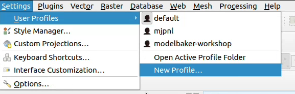
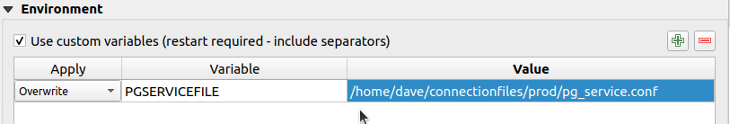
And you set the environment variable for each profile PGSERVICEFILE which should be used (in the menu Settings > Options… and there under System scroll down to Environment

or

If you now use the service my-local-gis in a QGIS layer, it connects the database prod in the “Prod” profile and the database test in the “Test” profile.

The authentication configuration

Let’s have a look at the authentication. If you have the connection service file on a network drive and make it available to several users, you may not want everyone to access it with the same login. Or you generally don’t want any user information in this file. This can be elegantly combined with the authentication configuration in QGIS.

If you want to make a QGIS project file available to multiple users, you create the layers with a service. This service contains all connection parameters except the login information.

This login information is transferred using QGIS authentication.

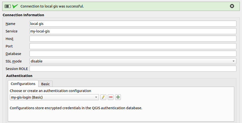
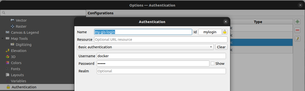
You also configure this authentication per QGIS profile we mentioned above. This is done via Menu Settings > Options… and there under Authentication:

(or directly where you create the PostgreSQL connection)

If you add such a layer, the service and the ID of the authentication configuration are saved in the QGIS project file. This is in this case mylogin. Of course this name must be communicated to the other users so that they can also set  the ID for their login to mylogin.

Of course, you can use multiple authentication configurations per profile.

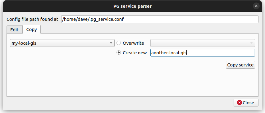
QGIS Plugin

And yes, there is now a great plugin to configure these services directly in QGIS. This means you no longer have to deal with text-based INI files. It’s called PG service parser:

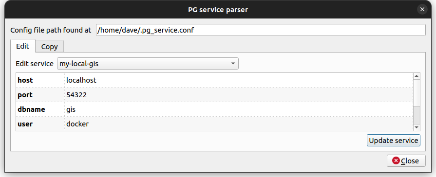
It finds the connection service file according to the mentioned environment variables PGSERVICEFILE or PGSYSCONFDIR or at its default location.

As well it’s super easy to create new services by duplicating existing ones.

And for the Devs

And what would a blog post be without some geek food? The back end of this plugin is published on PYPI and can be easily installed with pip install pgserviceparser and then be used in Python.

For example to list all the service names. 

>>> import pgserviceparser
>>> pgserviceparser.service_names()
['my-local-gis', 'another-local-gis', 'opengisch-demo-pg']

Optionally you can pass a config file path. Otherwise it gets it by the mentioned mechanism.

Or to receive the configuration from the given service name as a dict.

>>> pgserviceparser.service_config('my-local-gis')
{'host': 'localhost', 'port': '54322', 'dbname': 'gis', 'user': 'docker', 'password': 'docker'}

There are some more functions. Check them out here on GitHub or in the documentation.

Well then

We hope you share our enthusiasm for this beautiful file – at least after reading this blog post. And if not – feel free to tell us why you don’t in the comments 

Sorry, this entry is only available in French.

Sorry, this entry is only available in French.

Sorry, this entry is only available in French.

Recently there has been some buzz on Twitter about a new moving object database (MOD) called MobilityDB that builds on PostgreSQL and PostGIS (Zimányi et al. 2019). The MobilityDB Github repo has been published in February 2019 but according to the following presentation at PgConf.Russia 2019 it has been under development for a few years:

Of course, moving object databases have been around for quite a while. The two most commonly cited MODs are HermesDB (Pelekis et al. 2008) which comes as an extension for either PostgreSQL or Oracle and is developed at the University of Piraeus and SECONDO (de Almeida et al. 2006) which is a stand-alone database system developed at the Fernuniversität Hagen. However, both MODs remain at the research prototype level and have not achieved broad adoption.

It will be interesting to see if MobilityDB will be able to achieve the goal they have set in the title of Zimányi et al. (2019) to become “a mainstream moving object database system”. It’s promising that they are building on PostGIS and using its mature spatial analysis functionality instead of reinventing the wheel. They also discuss why they decided that PostGIS trajectories (which I’ve written about in previous posts) are not the way to go:

However, the presentation does not go into detail whether there are any straightforward solutions to visualizing data stored in MobilityDB.

According to the Github readme, MobilityDB runs on Linux and needs PostGIS 2.5. They also provide an online demo as well as a Docker container with MobilityDB and all its dependencies. If you give it a try, I would love to hear about your experiences.

References

• de Almeida, V. T., Guting, R. H., & Behr, T. (2006). Querying moving objects in secondo. In 7th International Conference on Mobile Data Management (MDM’06) (pp. 47-47). IEEE.
• Pelekis, N., Frentzos, E., Giatrakos, N., & Theodoridis, Y. (2008). HERMES: aggregative LBS via a trajectory DB engine. In Proceedings of the 2008 ACM SIGMOD international conference on Management of data (pp. 1255-1258). ACM.
• Zimányi, E., Sakr, M., Lesuisse, A., & Bakli, M. (2019). MobilityDB: A Mainstream Moving Object Database System. In Proceedings of the 16th International Symposium on Spatial and Temporal Databases (pp. 206-209). ACM.

This post is part of a series. Read more about movement data in GIS.

QGIS-versioning is a QGIS and PostGIS plugin dedicated to data versioning and history management. It supports :

• Keeping full table history with all modifications
• Transparent access to current data
• Versioning tables with branches
• Work offline
• Work on a data subset
• Conflict management with a GUI

QGIS versioning conflict management

In a previous blog article we detailed how QGIS versioning can manage data history, branches, and work offline with PostGIS-stored data and QGIS. We recently added foreign key support to QGIS versioning so you can now historize any complex database schema.

This QGIS plugin is available in the official QGIS plugin repository, and you can fork it on GitHub too !

Foreign key support

TL;DR

When a user decides to historize its PostgreSQL database with QGIS-versioning, the plugin alters the existing database schema and adds new fields in order to track down the different versions of a single table row. Every access to these versioned tables are subsequently made through updatable views in order to automatically fill in the new versioning fields.

Up to now, it was not possible to deal with primary keys and foreign keys : the original tables had to be constraints-free.  This limitation has been lifted thanks to this contribution.

To make it simple, the solution is to remove all constraints from the original database and transform them into a set of SQL check triggers installed on the working copy databases (SQLite or PostgreSQL). As verifications are made on the client side, it’s impossible to propagate invalid modifications on your base server when you “commit” updates.

Behind the curtains

When you choose to historize an existing database, a few fields are added to the existing table. Among these fields, versioning_ididentifies  one specific version of a row. For one existing row, there are several versions of this row, each with a different versioning_id but with the same original primary key field. As a consequence, that field cannot satisfy the unique constraint, so it cannot be a key, therefore no foreign key neither.

We therefore have to drop the primary key and foreign key constraints when historizing the table. Before removing them, constraints definitions are stored in a dedicated table so that these constraints can be checked later.

When the user checks out a specific table on a specific branch, QGIS-versioning uses that constraint table to build constraint checking triggers in the working copy. The way constraints are built depends on the checkout type (you can checkout in a SQLite file, in the master PostgreSQL database or in another PostgreSQL database).

What do we check ?

That’s where the fun begins ! The first thing we have to check is key uniqueness or foreign key referencing an existing key on insert or update. Remember that there are no primary key and foreign key anymore, we dropped them when activating historization. We keep the term for better understanding.

You also have to deal with deleting or updating a referenced row and the different ways of propagating the modification : cascade, set default, set null, or simply failure, as explained in PostgreSQL Foreign keys documentation .

Nevermind all that, this problem has been solved for you and everything is done automatically in QGIS-versioning. Before you ask, yes foreign keys spanning on multiple fields are also supported.

What’s new in QGIS ?

You will get a new message you probably already know about, when you try to make an invalid modification committing your changes to the master database

Error when foreign key constraint is violated

Partial checkout

One existing Qgis-versioning feature is partial checkout. It allows a user to select a subset of data to checkout in its working copy. It avoids downloading gigabytes of data you do not care about. You can, for instance, checkout features within a given spatial extent.

So far, so good. But if you have only a part of your data, you cannot ensure that modifying a data field as primary key will keep uniqueness. In this particular case, QGIS-versioning will trigger errors on commit, pointing out the invalid rows you have to modify so the unique constraint remains valid.

Error when committing non unique key after a partial checkout

Tests

There is a lot to check when you intend to replace the existing constraint system with your own constraint system based on triggers. In order to ensure QGIS-Versioning stability and reliability, we put some special effort on building a test set that cover all use cases and possible exceptions.

What’s next

There is now no known limitations on using QGIS-versioning on any of your database. If you think about a missing feature or just want to know more about QGIS and QGIS-versioning, feel free to contact us at [email protected]. And please have a look at our support offering for QGIS.

Many thanks to eHealth Africa who helped us develop these new features. eHealth Africa is a non-governmental organization based in Nigeria. Their mission is to build stronger health systems through the design and implementation of data-driven solutions.

Continuing our love story with PostgreSQL and QGIS, we asked QGIS.org a grant application during early 2017 spring.

The idea was to take benefit of very advanced PostgreSQL features, that probably never were used in a Desktop GIS client before.

Today, let’s see what we can do with the PostgreSQL NOTIFY feature!

Ever dreamt of being able to trigger things from outside QGIS? Ever wanted a magic stick to trigger actions in some clients from a database action?

NOTIFY is a PostgreSQL specific feature allowing to generate notifications on a channel and optionally send a message — a payload in PG’s dialect .

In short, from within a transaction, we can raise a signal in a PostgreSQL queue and listen to it from a client.

In action

We hardcoded a channel named “qgis” and made QGIS able to LISTEN to NOTIFY events and transform them into Qt’s signals. The signals are connected to layer refresh when you switch on this rendering option.

Optionnally, adding a message filter will only redraw the layer for some specific events.

This mechanism is really versatile and we now can imagine many possibilities, maybe like trigger a notification message to your users from the database, interact with plugins, or even code a chat between users of the same database  (ok, this is stupid) !

More than just refresh layers?

The first implementation we chose was to trigger a layer refresh because we believe this is a good way for users to discover this new feature.

But QGIS rocks hey, doing crazy things for limited uses is not the way.

Thanks to feedback on the Pull Request, we added the possibility to trigger layer actions on notification.

That should be pretty versatile since you can do almost anything with those actions now.

Caveats

QGIS will open a permanent connection to PostgreSQL to watch the notify signals. Please keep that in mind if you have several clients and a limited number of connections.

Notify signals are only transmitted with the transaction, so when the COMMIT is raised. So be aware that this might not help you if users are inside an edit session.

QGIS has a lot of different caches, for attribute table for instance. We currently have no specific way to invalidate a specific cache, and then order QGIS to refresh it’s attribute table.

There is no way in PG to list all channels of a database session, that’s why we couldn’t propose a combobox list of available signals in the renderer option dialog. Anyway, to avoid too many issues, we decided to hardcode the channel name in QGIS with the name “qgis”. If this is somehow not enough for your needs, please contact us!

Conclusion

The github pull request is here : https://github.com/qgis/QGIS/pull/5179

We are convinced this would be really useful for real time application, let us know if that makes some bells ring on your side!

More to come soon, stay tuned!

Let’s keep on looking at what we did in QGIS.org grant application of early 2017 spring.

At Oslandia, we use a lot the transaction groups option of QGIS. It was an experimental feature in QGIS 2.X allowing to open only one common Postgres transaction for all layers sharing the same connection string.

Transaction group option

When activated, that option will bring many killer features:

• Users can switch all the layers in edit mode at once. A real time saver.
• Every INSERT, UPDATE or DELETE is forwarded immediately to the database, which is nice for:
  • Evaluating on the fly if database constraints are satisfied or not. Without transaction groups this is only done when saving the edits and this can be frustrating to create dozens of features and having one of them rejected because of a foreign key constraint…
  • Having triggers evaluated on the fly.  QGIS is so powerful when dealing with “thick database” concepts that I would never go back to a pure GIS ignoring how powerful databases can be !
  • Playing with QgsTransaction.ExecuteSQL allows to trigger stored procedures in PostgreSQL in a beautiful API style interface. Something like

SELECT invert_pipe_direction('pipe1');

• However, the implementation was flagged “experimental” because some caveats where still causing issues:
  • Committing on the fly was breaking the logic of the undo/redo stack. So there was no way to do a local edit. No Ctrl+Z!  The only way to rollback was to stop the edit session and loose all the work. Ouch.. Bad!
  • Playing with ExecuteSQL did not dirty the QGIS edit buffer. So, if during an edit session no edit action was made using QGIS native tools, there was no clean way to activate the “save edits” icon.
  • When having some failures in the triggers, QGIS may loose DB connection and thus create a silent ROLLBACK.

We decided to try to restore the undo/redo stack by saving the history edits in PostgreSQL SAVEPOINTS and see if we could restore the original feature in QGIS.

And.. it worked!

Let’s see that in action:

Potential caveats ?

At start, we worried about how heavy all those savepoints would be for the database. It turns out that maybe for really massive geometries, and heavy editing sessions, this could start to weight a bit, but honestly far away from PostgreSQL capabilities.

Up to now, we didn’t really find any issue with that..

And we didn’t address the silent ROLLBACK that occurs sometimes, because it is generated by buggy stored procedures, easy to solve.

Some new ideas came to us when working in that area. For instance, if a transaction locks a feature, QGIS just… wait for the lock to be released. I think we should find a way to advertise those locks to the users, that would be great! If you’re interested in making that happen, please contact us.

More to come soon, stay tuned!

This is a guest post by Chris Kohler @Chriskohler8.

Introduction:

This guide provides step-by-step instructions to produce drive-time isochrones using a single vector shapefile. The method described here involves building a routing network using a single vector shapefile of your roads data within a Virtual Box. Furthermore, the network is built by creating start and end nodes (source and target nodes) on each road segment. We will use Postgresql, with PostGIS and Pgrouting extensions, as our database. Please consider this type of routing to be fair, regarding accuracy, as the routing algorithms are based off the nodes locations and not specific addresses. I am currently working on an improved workflow to have site address points serve as nodes to optimize results. One of the many benefits of this workflow is no financial cost to produce (outside collecting your roads data). I will provide instructions for creating, and using your virtual machine within this guide.

Steps:–Getting Virtual Box(begin)–

Intro 1. Download/Install Oracle VM(https://www.virtualbox.org/wiki/Downloads)

Intro 2. Start the download/install OSGeo-Live 11(https://live.osgeo.org/en/overview/overview.html).

Pictures used in this workflow will show 10.5, though version 11 can be applied similarly. Make sure you download the version: osgeo-live-11-amd64.iso. If you have trouble finding it, here is the direct link to the download (https://sourceforge.net/projects/osgeo-live/files/10.5/osgeo-live-10.5-amd64.iso/download)
Intro 3. Ready for virtual machine creation: We will utilize the downloaded OSGeo-Live 11 suite with a virtual machine we create to begin our workflow. The steps to create your virtual machine are listed below. Also, here are steps from an earlier workshop with additional details with setting up your virtual machine with osgeo live(http://workshop.pgrouting.org/2.2.10/en/chapters/installation.html).

1.  Create Virutal Machine: In this step we begin creating the virtual machine housing our database.

Open Oracle VM VirtualBox Manager and select “New” located at the top left of the window.

Then fill out name, operating system, memory, etc. to create your first VM.

2. Add IDE Controller:  The purpose of this step is to create a placeholder for the osgeo 11 suite to be implemented. In the virtual box main window, right-click your newly-created vm and open the settings.

In the settings window, on the left side select the storage tab.

Find “adds new storage controller” button located at the bottom of the tab. Be careful of other buttons labeled “adds new storage attachment”! Select “adds new storage controller” button and a drop-down menu will appear. From the top of the drop-down select “Add IDE Controller”.

You will see a new item appear in the center of the window under the “Storage Tree”.

3.  Add Optical Drive: The osgeo 11 suite will be implemented into the virtual machine via an optical drive. Highlight the new controller IDE you created and select “add optical drive”.

A new window will pop-up and select “Choose Disk”.

Locate your downloaded file “osgeo-live 11 amd64.iso” and click open. A new object should appear in the middle window under your new controller displaying “osgeo-live-11.0-amd64.iso”.

Finally your virtual machine is ready for use.
Start your new Virtual Box, then wait and follow the onscreen prompts to begin using your virtual machine.

–Getting Virtual Box(end)—

4. Creating the routing database, and both extensions (postgis, pgrouting): The database we create and both extensions we add will provide the functions capable of producing isochrones.

To begin, start by opening the command line tool (hold control+left-alt+T) then log in to postgresql by typing “psql -U user;” into the command line and then press Enter. For the purpose of clear instruction I will refer to database name in this guide as “routing”, feel free to choose your own database name. Please input the command, seen in the figure below, to create the database:

CREATE DATABASE routing;

You can use “\c routing” to connect to the database after creation.

The next step after creating and connecting to your new database is to create both extensions. I find it easier to take two-birds-with-one-stone typing “psql -U user routing;” this will simultaneously log you into postgresql and your routing database.

When your logged into your database, apply the commands below to add both extensions

CREATE EXTENSION postgis;
CREATE EXTENSION pgrouting;

5. Load shapefile to database: In this next step, the shapefile of your roads data must be placed into your virtual machine and further into your database.

My method is using email to send myself the roads shapefile then download and copy it from within my virtual machines web browser. From the desktop of your Virtual Machine, open the folder named “Databases” and select the application “shape2pgsql”.

Follow the UI of shp2pgsql to connect to your routing database you created in Step 4.

Next, select “Add File” and find your roads shapefile (in this guide we will call our shapefile “roads_table”) you want to use for your isochrones and click Open.

Finally, click “Import” to place your shapefile into your routing database.

6. Add source & target columns: The purpose of this step is to create columns which will serve as placeholders for our nodes data we create later.

There are multiple ways to add these columns into the roads_table. The most important part of this step is which table you choose to edit, the names of the columns you create, and the format of the columns. Take time to ensure the source & target columns are integer format. Below are the commands used in your command line for these functions.

ALTER TABLE roads_table ADD COLUMN "source" integer;
ALTER TABLE roads_table ADD COLUMN "target" integer;

7. Create topology: Next, we will use a function to attach a node to each end of every road segment in the roads_table. The function in this step will create these nodes. These newly-created nodes will be stored in the source and target columns we created earlier in step 6.

As well as creating nodes, this function will also create a new table which will contain all these nodes. The suffix “_vertices_pgr” is added to the name of your shapefile to create this new table. For example, using our guide’s shapefile name , “roads_table”, the nodes table will be named accordingly: roads_table_vertices_pgr. However, we will not use the new table created from this function (roads_table_vertices_pgr). Below is the function, and a second simplified version, to be used in the command line for populating our source and target columns, in other words creating our network topology. Note the input format, the “geom” column in my case was called “the_geom” within my shapefile:

pgr_createTopology('roads_table', 0.001, 'geom', 'id',
 'source', 'target', rows_where := 'true', clean := f)

Here is a direct link for more information on this function: http://docs.pgrouting.org/2.3/en/src/topology/doc/pgr_createTopology.html#pgr-create-topology

Below is an example(simplified) function for my roads shapefile:

SELECT pgr_createTopology('roads_table', 0.001, 'the_geom', 'id')

8. Create a second nodes table: A second nodes table will be created for later use. This second node table will contain the node data generated from pgr_createtopology function and be named “node”. Below is the command function for this process. Fill in your appropriate source and target fields following the manner seen in the command below, as well as your shapefile name.

To begin, find the folder on the Virtual Machines desktop named “Databases” and open the program “pgAdmin lll” located within.

Connect to your routing database in pgAdmin window. Then highlight your routing database, and find “SQL” tool at the top of the pgAdmin window. The tool resembles a small magnifying glass.

We input the below function into the SQL window of pgAdmin. Feel free to refer to this link for further information: (https://anitagraser.com/2011/02/07/a-beginners-guide-to-pgrouting/)

CREATE TABLE node AS
   SELECT row_number() OVER (ORDER BY foo.p)::integer AS id,
          foo.p AS the_geom
   FROM (     
      SELECT DISTINCT roads_table.source AS p FROM roads_table
      UNION
      SELECT DISTINCT roads_table.target AS p FROM roads_table
   ) foo
   GROUP BY foo.p;

9.  Create a routable network: After creating the second node table from step 8,  we will combine this node table(node) with our shapefile(roads_table) into one, new, table(network) that will be used as the routing network. This table will be called “network” and will be capable of processing routing queries.  Please input this command and execute in SQL pgAdmin tool as we did in step 8. Here is a reference for more information:(https://anitagraser.com/2011/02/07/a-beginners-guide-to-pgrouting/)   

CREATE TABLE network AS
   SELECT a.*, b.id as start_id, c.id as end_id
   FROM roads_table AS a
      JOIN node AS b ON a.source = b.the_geom
      JOIN node AS c ON a.target = c.the_geom;

10. Create a “noded” view of the network:  This new view will later be used to calculate the visual isochrones in later steps. Input this command and execute in SQL pgAdmin tool.

CREATE OR REPLACE VIEW network_nodes AS 
SELECT foo.id,
 st_centroid(st_collect(foo.pt)) AS geom 
FROM ( 
  SELECT network.source AS id,
         st_geometryn (st_multi(network.geom),1) AS pt 
  FROM network
  UNION 
  SELECT network.target AS id, 
         st_boundary(st_multi(network.geom)) AS pt 
  FROM network) foo 
GROUP BY foo.id;

11.​ Add column for speed:​ This step may, or may not, apply if your original shapefile contained a field of values for road speeds.

In reality a network of roads will typically contain multiple speed limits. The shapefile you choose may have a speed field, otherwise the discrimination for the following steps will not allow varying speeds to be applied to your routing network respectfully.

If values of speed exists in your shapefile we will implement these values into a new field, “traveltime“, that will show rate of travel for every road segment in our network based off their geometry. Firstly, we will need to create a column to store individual traveling speeds. The name of our column will be “traveltime” using the format: ​double precision.​ Input this command and execute in the command line tool as seen below.

ALTER TABLE network ADD COLUMN traveltime double precision;

Next, we will populate the new column “traveltime” by calculating traveling speeds using an equation. This equation will take each road segments geometry(shape_leng) and divide by the rate of travel(either mph or kph). The sample command I’m using below utilizes mph as the rate while our geometry(shape_leng) units for my roads_table is in feet​. If you are using either mph or kph, input this command and execute in SQL pgAdmin tool. Below further details explain the variable “X”.

UPDATE network SET traveltime = shape_leng / X*60

How to find X​, ​here is an example​: Using example 30 mph as rate. To find X, we convert 30 miles to feet, we know 5280 ft = 1 mile, so we multiply 30 by 5280 and this gives us 158400 ft. Our rate has been converted from 30 miles per hour to 158400 feet per hour. For a rate of 30 mph, our equation for the field “traveltime”  equates to “shape_leng / 158400*60″. To discriminate this calculations output, we will insert additional details such as “where speed = 30;”. What this additional detail does is apply our calculated output to features with a “30” value in our “speed” field. Note: your “speed” field may be named differently.

UPDATE network SET traveltime = shape_leng / 158400*60 where speed = 30;

Repeat this step for each speed value in your shapefile examples:

UPDATE network SET traveltime = shape_leng / X*60 where speed = 45;
UPDATE network SET traveltime = shape_leng / X*60 where speed = 55;

The back end is done. Great Job!

Our next step will be visualizing our data in QGIS. Open and connect QGIS to your routing database by right-clicking “PostGIS” in the Browser Panel within QGIS main window. Confirm the checkbox “Also list tables with no geometry” is checked to allow you to see the interior of your database more clearly. Fill out the name or your routing database and click “OK”.

If done correctly, from QGIS you will have access to tables and views created in your routing database. Feel free to visualize your network by drag-and-drop the network table into your QGIS Layers Panel. From here you can use the identify tool to select each road segment, and see the source and target nodes contained within that road segment. The node you choose will be used in the next step to create the views of drive-time.

12. ​Create views​: In this step, we create views from a function designed to determine the travel time cost. Transforming these views with tools will visualize the travel time costs as isochrones.

The command below will be how you start querying your database to create drive-time isochrones. Begin in QGIS by draging your network table into the contents. The visual will show your network as vector(lines). Simply select the road segment closest to your point of interest you would like to build your isochrone around. Then identify the road segment using the identify tool and locate the source and target fields. ​

Place the source or target field value in the below command where you see ​VALUE​, in all caps​.

This will serve you now as an isochrone catchment function for this workflow. Please feel free to use this command repeatedly for creating new isochrones by substituting the source value. Please input this command and execute in SQL pgAdmin tool.

*AT THE BOTTOM OF THIS WORKFLOW I PROVIDED AN EXAMPLE USING SOURCE VALUE “2022”

CREATE OR REPLACE VIEW "​view_name" AS 
SELECT di.seq, 
       di.id1, 
       di.id2, 
       di.cost, 
       pt.id, 
       pt.geom 
FROM pgr_drivingdistance('SELECT
     gid::integer AS id, 
     Source::integer AS source, 
     Target::integer AS target,                                    
     Traveltime::double precision AS cost 
       FROM network'::text, ​VALUE::bigint, 
    100000::double precision, false, false)
    di(seq, id1, id2, cost)
JOIN network_nodes pt ON di.id1 = pt.id;

13. ​Visualize Isochrone: Applying tools to the view will allow us to adjust the visual aspect to a more suitable isochrone overlay.

​After creating your view, a new item in your routing database is created, using the “view_name” you chose. Drag-and-drop this item into your QGIS LayersPanel. You will see lots of small dots which represent the nodes.

In the figure below, I named my view “take1“.

Each node you see contains a drive-time value, “cost”, which represents the time used to travel from the node you input in step 12’s function.

Start by installing the QGIS plug-in “Interpolation” by opening the Plugin Manager in QGIS interface.

Next, at the top of QGIS window select “Raster” and a drop-down will appear, select “Interpolation”.

A new window pops up and asks you for input.

Select your “​view”​ as the​ vector layer​, select ​”cost​” as your ​interpolation attribute​, and then click “Add”.

A new vector layer will show up in the bottom of the window, take care the type is “Points“. For output, on the other half of the window, keep the interpolation method as “TIN”, edit the ​output file​ location and name. Check the box “​Add result to project​”.

Note: decreasing the cellsize of X and Y will increase the resolution but at the cost of performance.

Click “OK” on the bottom right of the window.

A black and white raster will appear in QGIS, also in the Layers Panel a new item was created.

Take some time to visualize the raster by coloring and adjusting values in symbology until you are comfortable with the look.

14. ​Create contours of our isochrone:​ Contours can be calculated from the isochrone as well.

Find near the top of QGIS window, open the “Raster” menu drop-down and select Extraction → Contour.

Fill out the appropriate interval between contour lines but leave the check box “Attribute name” unchecked. Click “OK”.

15.​ Zip and Share:​ Find where you saved your TIN and contours, compress them in a zip folder by highlighting them both and right-click to select “compress”. Email the compressed folder to yourself to export out of your virtual machine.

Example Isochrone catchment for this workflow:

CREATE OR REPLACE VIEW "2022" AS 
SELECT di.seq, Di.id1, Di.id2, Di.cost,                           
       Pt.id, Pt.geom 
FROM pgr_drivingdistance('SELECT gid::integer AS id,                                       
     Source::integer AS source, Target::integer AS target, 
     Traveltime::double precision AS cost FROM network'::text, 
     2022::bigint, 100000::double precision, false, false) 
   di(seq, id1, id2, cost) 
JOIN netowrk_nodes pt 
ON di.id1 = pt.id;

References: Virtual Box ORACLE VM, OSGeo-Live 11  amd64 iso, Workshop FOSS4G Bonn(​http://workshop.pgrouting.org/2.2.10/en/index.html​),

This post is a quick instruction for installing Postgres 9.2, PostGIS 2.0 and pgRouting 2.0.

1. For Postgres, download the installer from enterprisedb.com.
2. Run the installer. You’ll have to pick a superuser password – remember it, you’ll need it again soon.
3. At the end of the installation process, allow the installer to start Stack Builder.
4. In Stack Builder, select the Postgres 9.2 installation and install PostGIS from the list of available extensions.
5. The PostGIS installation procedure will prompt you for the superuser password you picked before.
6. I suggest letting the installer create a sample database We’ll need it later anyway.

Now for the pgRouting part:

1. Download the pgRouting zip file for your system (32 or 64 bit) from Winnie.
2. Unzip the file. It contains bin, lib and share folders as well as two text files.
3. Copy these folders and files over to your Postgres installation. In my case C:\Program Files\PostgreSQL\9.2

Installation – done.

Next, fire up pgAdmin. If you allowed the PostGIS installer to create a sample database, you will find it named postgis20 or similar. Otherwise just create a new database using the PostGIS template database. You can enable pgRouting in a database using the following steps:

1. In postgis20, execute the following query to create the pgrouting extension. This will add the pgRouting-specific functions:

   CREATE EXTENSION pgrouting;

2. Test if everything worked fine:

   SELECT pgr_version();

   It should return "(2.0.0-dev,v2.0.0-beta,18,a3be38b,develop,1.46.1)" or similar – depending on the version you downloaded.

How about some test data? I’ll be using the public transport network of the city of Vienna provided in GeoJSON format from http://data.wien.gv.at/daten/wfs?service=WFS&request=GetFeature&version=1.1.0&typeName=ogdwien:OEFFLINIENOGD&srsName=EPSG:4326&outputFormat=json:

1. Just copy paste the url in Add Vector Layer | Protocol to load the dataset.
2. Use DB Manager to load the layer into your database. (As you can see in the screenshot, I created a schema called network but that’s optional.)



3. To make the line vector table routable, we use pgr_createTopology. This function assumes the columsn called “source” and “target” exist so we have to create those as well:

   alter table network.publictransport add column source integer;
   alter table network.publictransport add column target integer;
   select pgr_createTopology('network.publictransport', 0.0001, 'geom', 'id');
   

   I’m quite generously using a tolerance of 0.0001 degrees to build the topology. Depending on your dataset, you might want to be more strict here.

4. Let’s test it! Route from source #1 to target #3000 using pgr_dijkstra:

   SELECT seq, id1 AS node, id2 AS edge, cost, geom
     FROM pgr_dijkstra(
       'SELECT id, source, target, st_length(geom) as cost FROM network.publictransport',
       1, 3000, false, false
     ) as di
     JOIN network.publictransport pt
     ON di.id2 = pt.id ;

   Note how the query joins the routing results and the network table together. (I’m aware that using the link length as a cost attribute will not lead to realistic results in a public transport network but bear with me for this example.)

5. We can immediately see the routing results using the Load as new layer option:

Nice work! pgRouting 2.0 has come a long way. In a post from April this year, Boston GIS even announced to add pgRouting into the Stack Builder. That’s going to make the installation even more smooth.

For everyone working with spatial databases in QGIS there comes a time when “Add PostGIS/SpatiaLite Layer” and “RT Sql Layer” start to be annoying. You always have to retype or copy-paste your SQL queries into the user interface if you need to change the tiniest thing in the layer’s definition.

This is where “Fast SQL Layer” can be a real time saver. Fast SQL Layer is a new plugin for QGIS by Pablo T. Carreira. It basically adds an SQL console for loading layers from PostGIS/SpatiaLite into QGIS. And it even comes with syntax highlighting!

Installation

Fast SQL Layer comes with one dependency: Pygments, which is used for syntax highlighting.

On Ubuntu, all you have to do is install it with apt-get:

sudo apt-get install python-pygments

For Windows with OSGeo4W, @Mike_Toews posted this on gis.stackexchange:

I downloaded and extracted Pygments-1.4.tar.gz, then in an OSGeo4W shell within the Pygments-1.4 directory, type python setup.py build then python setup.py install

Usage

When you activate the plugin in plugin manager, a dock widget will appear which contains the console and some fields for specifying the database connection that should be used. Then, you can simply write your SQL query and load the results with one click.

Fast SQL plugin

In this example, I renamed “gid” to “id”, but you can actually edit the values in the drop down boxes to adjust the column names for id and geometry:

A second layer loaded using Fast SQL plugin

It certainly needs some polishing on the user interface side but I really like it.

A while ago I’ve compiled PostGIS 1.5.2 for PostgreSQL 9.0.

To install it on Ubuntu the following steps are required:

apt-get install python-software-properties

add-apt-repository ppa:ubuntugis/ubuntugis-unstable
add-apt-repository ppa:pitti/postgresql
add-apt-repository ppa:pi-deb/gis

apt-get update

apt-get install postgresql-9.0-postgis

A basic template database can be created with the following commands:

sudo su - postgres

createdb template_postgis
psql -q -d template_postgis -f /usr/share/postgresql/9.0/contrib/postgis-1.5/postgis.sql
psql -q -d template_postgis -f /usr/share/postgresql/9.0/contrib/postgis-1.5/spatial_ref_sys.sql
psql -q -d template_postgis -f /usr/share/postgresql/9.0/contrib/postgis_comments.sql
cat <<EOS | psql -d template_postgis
UPDATE pg_database SET datistemplate = TRUE WHERE datname = 'template_postgis';
REVOKE ALL ON SCHEMA public FROM public;
GRANT USAGE ON SCHEMA public TO public;
GRANT ALL ON SCHEMA public TO postgres;
GRANT SELECT, UPDATE, INSERT, DELETE
  ON TABLE public.geometry_columns TO PUBLIC;
GRANT SELECT, UPDATE, INSERT, DELETE
  ON TABLE public.spatial_ref_sys TO PUBLIC;
EOS

To test database creation you can do the following:

createdb --template template_postgis test_gis
psql -d test_gis -c "select postgis_lib_version();"

Ubuntu supports parallel installations of different PostgreSQL versions. So if you have already PostgreSQL 8.x installed, PostgreSQL 9.0 will probably be configured to listen on port 5433. So you have to add the option -p 5433 to each command and to specify the full path for the executables. For example:

/usr/lib/postgresql/9.0/bin/psql -p 5433 -d test_gis -c "select postgis_lib_version();"

A while ago I’ve compiled PostGIS 1.5.2 for PostgreSQL 9.0.

To install it on Ubuntu the following steps are required:

apt-get install python-software-properties

add-apt-repository ppa:ubuntugis/ubuntugis-unstable
add-apt-repository ppa:pitti/postgresql
add-apt-repository ppa:pi-deb/gis

apt-get update

apt-get install postgresql-9.0-postgis

A basic template database can be created with the following commands:

sudo su - postgres

createdb template_postgis
psql -q -d template_postgis -f /usr/share/postgresql/9.0/contrib/postgis-1.5/postgis.sql
psql -q -d template_postgis -f /usr/share/postgresql/9.0/contrib/postgis-1.5/spatial_ref_sys.sql
psql -q -d template_postgis -f /usr/share/postgresql/9.0/contrib/postgis_comments.sql
cat <<EOS | psql -d template_postgis
UPDATE pg_database SET datistemplate = TRUE WHERE datname = 'template_postgis';
REVOKE ALL ON SCHEMA public FROM public;
GRANT USAGE ON SCHEMA public TO public;
GRANT ALL ON SCHEMA public TO postgres;
GRANT SELECT, UPDATE, INSERT, DELETE
  ON TABLE public.geometry_columns TO PUBLIC;
GRANT SELECT, UPDATE, INSERT, DELETE
  ON TABLE public.spatial_ref_sys TO PUBLIC;
EOS

To test database creation you can do the following:

createdb --template template_postgis test_gis
psql -d test_gis -c "select postgis_lib_version();"

Ubuntu supports parallel installations of different PostgreSQL versions. So if you have already PostgreSQL 8.x installed, PostgreSQL 9.0 will probably be configured to listen on port 5433. So you have to add the option -p 5433 to each command and to specify the full path for the executables. For example:

/usr/lib/postgresql/9.0/bin/psql -p 5433 -d test_gis -c "select postgis_lib_version();"

Today’s challenge is to read data from a CSV file and construct usable timestamps. This is the layout of the file, notice the missing leading zeros in the month, hour and seconds fields:

utc_date;utc_time
"2011/3/15 ";"6:17:3 "
"2011/3/15 ";"6:17:8 "
"2011/3/15 ";"6:17:13 "
"2011/3/15 ";"6:17:18 "
"2011/3/15 ";"6:17:23 "

To get the data into Postgres, I used the copy command with csv header option. The table has to exist already. “csv header” tells the command to ignore the file’s header line.

copy mytable
from '~/my.csv'
csv header;

Now, we have to handle the “missing leading zeros” problem. Luckily, Postgres offers a template pattern modifier that addresses exactly this problem: the “FM” (fill mode) prefix. The pattern for a month without leading zeros therefore is ‘FMMM’. The full to_timestamp command looks like this:

update mytable
set utc_timestamp = to_timestamp(utc_date||' '||utc_time,'YYYY/FMMM/FMDD FMHH24:FMMI:FMSS' )

Do you need a random sample of features in a Postgres table? Here is an example of how to select 1,000 random features from a table:

SELECT * FROM myTable
WHERE attribute = 'myValue'
ORDER BY random()
LIMIT 1000;

Besides many other interesting topics, Opengeo’s PostGIS tutorial discusses “Tuning PostgreSQL for Spatial”.

The following values are recommended for production environments:

• shared_buffers: 75 % of database memory (500 MB)
• work_mem: 16 MB
• maintenance_work_mem: 128 MB
• wal_buffers: 1 MB
• checkpoint_segments: 6
• random_page_cost: 2.0
• seq_page_cost: 1.0

All of these configuration parameters can edited in the database configuration file, C:\Documents and Settings\%USER\.opengeo\pgdata\%USER. This is a regular text file and can be edited using Notepad or any other text editor. An easier way of editing this configuration is by using the built-in “Backend Configuration Editor”. In pgAdmin, go to File > Open postgresql.conf…. It will ask for the location of the file, and navigate to C:\Documents and Settings\%USER\.opengeo\pgdata\%USER.

The changes will not take effect until the server is restarted.