Related Plugins and Tags

QGIS Planet

Spatial data exploration with linked plots

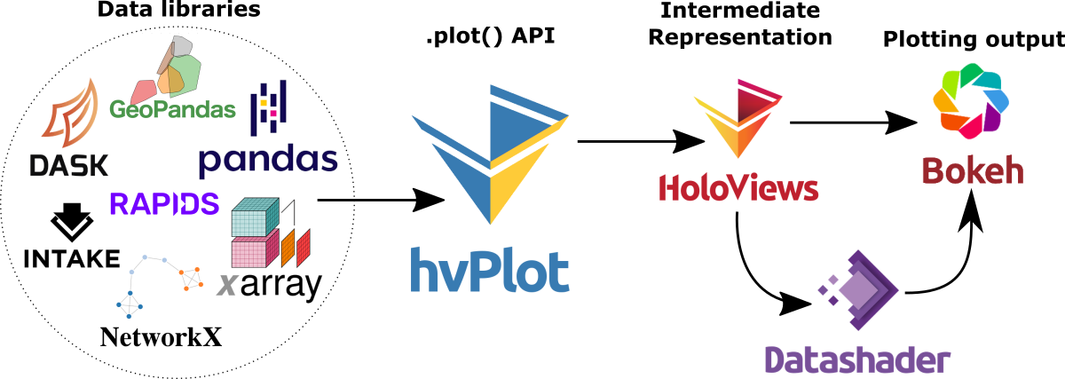
In the previous post, we explored how hvPlot and Datashader can help us to visualize large CSVs with point data in interactive map plots. Of course, the spatial distribution of points usually only shows us one part of the whole picture. Today, we’ll therefore look into how to explore other data attributes by linking other (non-spatial) plots to the map.

This functionality, referred to as “linked brushing” or “crossfiltering” is under active development and the following experiment was prompted by a recent thread on Twitter launched by @plotlygraphs announcement of HoloViews 1.14:

Turns out these features are not limited to plotly but can also be used with Bokeh and hvPlot:

Like in the previous post, this demo uses a Pandas DataFrame with 12 million rows (and HoloViews 1.13.4).

In addition to the map plot, we also create a histogram from the same DataFrame:

map_plot = df.hvplot.scatter(x='x', y='y', datashade=True, height=300, width=400)
hist_plot = df.where((df.SOG>0) & (df.SOG<50)).hvplot.hist("SOG",  bins=20, width=400, height=200) 

To link the two plots, we use HoloViews’ link_selections function:

from holoviews.selection import link_selections
linked_plots = link_selections(map_plot + hist_plot)

That’s all! We can now perform spatial filters in the map and attribute value filters in the histogram and the filters are automatically applied to the linked plots:

Linked brushing demo using ship movement data (AIS): filtering records by speed (SOG) reveals spatial patterns of fast and slow movement.

You’ve probably noticed that there is no background map in the above plot. I had to remove the background map tiles to get rid of an error in Holoviews 1.13.4. This error has been fixed in 1.14.0 but I ran into other issues with the datashaded Scatterplot.

It’s worth noting that not all plot types support linked brushing. For the complete list, please refer to http://holoviews.org/user_guide/Linked_Brushing.html

Plotting large point CSV files quickly & interactively

Even with all their downsides, CSV files are still a common data exchange format – particularly between disciplines with different tech stacks. Indeed, “How to Specify Data Types of CSV Columns for Use in QGIS” (originally written in 2011) is still one of the most popular posts on this blog. QGIS continues to be quite handy for visualizing CSV file contents. However, there are times when it’s just not enough, particularly when the number of rows in the CSV is in the range of multiple million. The following example uses a 12 million point CSV:

To give you an idea of the waiting times in QGIS, I’ve run the following script which loads and renders the CSV:

from datetime import datetime

def get_time():
    t2 = datetime.now()
    print(t2)
    print(t2-t1)
    print('Done :)')

canvas = iface.mapCanvas()
canvas.mapCanvasRefreshed.connect(get_time)

print('Starting ...')

t0 = datetime.now()
print(t0)

print('Loading CSV ...')

uri = "file:///E:/Geodata/AISDK/raw_ais/aisdk_20170701.csv?type=csv&amp;xField=Longitude&amp;yField=Latitude&amp;crs=EPSG:4326&amp;"
vlayer = QgsVectorLayer(uri, "layer name you like", "delimitedtext")

t1 = datetime.now()
print(t1)
print(t1 - t0)

print('Rendering ...')

QgsProject.instance().addMapLayer(vlayer)

The script output shows that creating the vector layer takes 02:39 minutes and rendering it takes over 05:10 minutes:

Starting ...
2020-12-06 12:35:56.266002
Loading CSV ...
2020-12-06 12:38:35.565332
0:02:39.299330
Rendering ...
2020-12-06 12:43:45.637504
0:05:10.072172
Done :)

Rendered CSV file in QGIS

Panning and zooming around are no fun either since rendering takes so long. Changing from a single symbol renderer to, for example, a heatmap renderer does not improve the rendering times. So we need a different solutions when we want to efficiently explore large point CSV files.

The Pandas data analysis library is well-know for being a convenient tool for handling CSVs. However, it’s less clear how to use it as a replacement for desktop GIS for exploring large CSVs with point coordinates. My favorite solution so far uses hvPlot + HoloViews + Datashader to provide interactive Bokeh plots in Jupyter notebooks.

hvPlot provides a high-level plotting API built on HoloViews that provides a general and consistent API for plotting data in (Geo)Pandas, xarray, NetworkX, dask, and others. (Image source: https://hvplot.holoviz.org)

But first things first! Loading the CSV as a Pandas Dataframe takes 10.7 seconds. Pandas’ default plotting function (based on Matplotlib), however, takes around 13 seconds and only produces a static scatter plot.

Loading and plotting the CSV with Pandas

hvPlot to the rescue!

We only need two more steps to get faster and interactive map plots (plus background maps!): First, we need to reproject the lat/lon values. (There’s a warning here, most likely since some of the input lat/lon values are invalid.) Then, we replace plot() with hvplot() and voilà:

Plotting the CSV with Datashader

As you can see from the above GIF, the whole process barely takes 2 seconds and the resulting map plot is interactive and very responsive.

12 million points are far from the limit. As long as the Pandas DataFrame fits into memory, we are good and when the datasets get bigger than that, there are Dask DataFrames. But that’s a story for another day.

  • Page 1 of 1 ( 2 posts )
  • datashader

Back to Top

Sustaining Members