QField 3.4 is out, and it won’t disappoint. It has tons of new features that continue to push the limits of what users can do in the field.
Main highlights
A new geofencing framework has landed, enabling users to configure QField behaviors in relation to geofenced areas and user positioning. Geofenced areas are defined at the project-level and shaped by polygons from a chosen vector layer. The three available geofencing behaviours in this new release are:
Alert user when inside an area polygon;
Alert user when outside all defined area polygons and
Inform the user when entering and leaving an area polygons.
In addition to being alerted or informed, users can also prevent digitizing of features when being alerted by the first or second behaviour. The configuration of this functionality is done in QGIS using QFieldSync.
Pro tip: geofencing settings are embedded within projects, which means it is easy to deploy these constraints to a team of field workers through QFieldCloud. Thanks Terrex Seismic for sponsoring this functionality.
QField now offers users access to a brand new processing toolbox containing over a dozen algorithms for manipulating digitized geometries directly in the field. As with many parts of QField, this feature relies on QGIS’ core library, namely its processing framework and the numerous, well-maintained algorithms it comes with.
The algorithms exposed in QField unlock many useful functionalities for refining geometries, including orthogonalization, smoothing, buffering, rotation, affine transformation, etc. As users configure algorithms’ parameters, a grey preview of the output will be visible as an overlay on top of the map canvas.
To reach the processing toolbox in QField, select one or more features by long-pressing on them in the features list, open the 3-dot menu and click on the process selected feature(s) action. Are you excited about this one? Send your thanks to the National Land Survey of Finland, who’s support made this a reality.
QField’s camera has gained support for customized ratio and resolution of photos, as well as the ability to stamp details – date and time as well as location details – onto captured photos. In fact, QField’s own camera has received so much attention in the last few releases that we have decided to make it the default one. On supported platforms, users can switch to their OS camera by disabling the native camera option found at the bottom of the QField settings’ general tab.
Wait, there’s more
There are plenty more improvements packed into this release from project variables editing using a revamped variables editor through to integration of QField documentation help in the search bar and the ability to search cloud project lists. Read the full 3.4 changelog to know more, and enjoy the release!
QField Rapid Mapper is a project for the QField mobile app, which allows emergency responders, civil protection, military, and citizens to assess and report damages from natural catastrophes by quickly sharing geolocated images, videos and audio. QField Rapid Mapper offers real-time data collection, mapping and sharing to help enhance disaster response and coordination. QField and QFieldCloud are open-source, and OPENGIS.ch is donating the needed QFieldCloud infrastructure and expertise to help map the floods in Ticino in 2024
OPENGIS.ch Supports Flood Mapping Efforts in Ticino
After discussing with the Protezione Civile Locarno e Valle Maggia and the Centro di Competenza per la geoinformazione (CCGEO), we are proud to announce that OPENGIS.ch is donating the necessary QFieldCloud infrastructure and dedicated projects for a rapid crowdsourcing POC to aid in mapping the 2024 floods in Ticino. This crowdsourcing initiative aims to provide essential support to professionals and volunteers working on flood and landslide assessment and recovery.
Photographing damaged houses and infrastructure is the most critical aspect of this mapping initiative. These images provide crucial information for assessing the extent of the damage, planning rescue and reconstruction operations, and ensuring that resources are allocated effectively. It’s also important to document any submerged or damaged vehicles, as they offer additional insights into the disaster’s impact. During these activities, it’s essential to be careful and respect the privacy and property of others, avoiding capturing license plate numbers or entering destroyed buildings without permission. Using QField Rapid Mapper can contribute to a faster and more coordinated emergency response while ensuring respect for those affected.
The QFieldCloud infrastructure enables efficient, real-time data collection and sharing, ensuring that accurate and up-to-date information is available to all stakeholders involved in the flood response. This effort underscores our commitment to leveraging technology for social good and environmental resilience.
By participating, you will have access to powerful tools for field data collection and can contribute valuable information to the ongoing efforts in Ticino. All the data collected will be released under the Creative Commons CC0 1.0 public domain license.
Join the Effort
Using QField and QFieldCloud, you can help create detailed maps crucial for understanding the impact of the floods and planning effective recovery strategies. Your contributions will make a significant difference in managing and mitigating the effects of this natural disaster.
Visit our QField Rapid Mapper project page for more information on how QField and QFieldCloud can assist in flood mapping and other field data collection projects.
Together, we can make a difference. Join us in mapping the floods in Ticino and support the community’s recovery efforts.
Get high-precision elevation profiles in QGIS right from Swisstopo’s official profile service, based on swissALTI3D data!
Swiss elevation profiles are available with QGIS 3.38.
Thanks to this integration, you can take advantage of existing QGIS features, such as exporting 2d/3d features or distance/elevation tables, as well as displaying profiles directly in QGIS layouts.
Tip: Swiss elevation profiles will be available as long as the Swiss Locator plugin is installed and active. Should you need to turn Swiss elevation profiles off to create other profiles with your own data, go to the Plugin manager and deactivate the plugin in the meantime.
For developers
We’re paving the way for adding custom elevation profiles to QGIS. For that, we’ve added a QGIS profile source registry so that plugin developers can register their own profile sources (e.g., based on profile web services, just like we did here) and make them available for QGIS end users. The registry is available from QGIS 3.38. It’s your turn!
Loading Swiss vector tiles is now easier than ever. Just go to the locator bar, type the prefix “chb” (add a white space after that) and you’ll get a list of available and already styled Swiss vector tiles layers. Some of them will even load grouped auxiliary imagery for reference.
Vector tiles will be loaded at the bottom of the QGIS layer tree as base maps, so you will see all your data on top of them.
Vector tiles are optimized for local caching and scale-independent rendering. This also makes it a perfect fit for adding it to your QField project.
There are a couple of different vector tile sets available:
leichte-basiskarte
Light base map
Similar to the leichte-basiskarte layer, but using an older version of the data source and adjusted styles.
leichte-basiskarte-imagery (with WMTS sublayer)
Imagery base map (with WMTS sublayer)
This layer is similar to the leichte-basiskarte-imagery layer, but it uses an older version of the data source and adjusted styles.
Thanks to your feedback, we’ve also fixed some issues. Don’t hesitate to reach out to us at GitHub if you’d like to suggest or report something related to the Swiss Locator plugin.
During the pandemic, people noticed how well they could work remotely, how productive meetings via video call could be, and how well webinars worked. At OPENGIS.ch, this wasn’t news because we have always been 100% remote. However, we missed the unplanned, in-person interactions that occur during meetups with a or . That’s why we’re very pleased that last week we could join the Swiss QGIS user day for the second time after the pandemic.
OPENGIS.ch has been invested in QGIS since its inception in 2014, actually even before; our CEO Marco started working with QGIS 0.6 in 2004 and our CTO Matthias with version 1.7 in 2012. Since 2019, we have also been the company with the most core committers. We can definitely say that OPENGIS.ch has been one of the main driving forces behind the large adoption of QGIS in Switzerland and worldwide.
Contributions to the QGIS core measured in commit numbers
Looking at the work done in the QGIS code we’re by far the most prolific company in Switzerland and second worldwide only to North Road Consulting. On top of it, we were the first – and still only one of two- companies to sustain QGIS.org at a Large level since 2021.
This makes us very proud and it is why we’re even happier to see how much that is happening around QGIS in Switzerland aligns with the visions and goals we set out to reach years ago.
The morning started with a presentation by our CTO Matthias “What’s new in QGIS” featuring plenty of work sponsored by the Anwendergruppe CH.
Our CTO Matthias answering QGIS questions
DXF Improvements, the release of SwissLocator 3.0 with swissalti3d and vector tiles integration, and an update on the advances towards solid curve handling in QGIS, a prerequisite for properly handling AV data in Switzerland, were only some of the many noteworthy points he touched.
The highlight of Matthias’ presentation was the better OGC API Features support in QGIS, which was also highlighted in a subsequent talk about Kablo, showing how the next generation of industry solutions (Fachschalen) will be implemented.
Following was a short presentation on the project DMAV, Christoph Lauber introduced a project that aims to implement an industry solution for official cadastral surveying with QGIS.
Adrian Wicki of the Federal Office for the Environment (FOEN) and Isabel presented how OPENGIS.ch and the partners Puzzle and Zeilenwerk help the FOEN with the SAM project with assess the hazards of flood, forest fire, or landslides, and warn authorities and the population. With an agile project organisation, the complex project succeeds in fulfilling requirements by applying user-centred development concepts. QGIS is used for visualizing and analyzing data and helping forecasters gain insights into the current situation.
Andreas Neumann from ETH Zurich and Michael presented the qgis-js project. QGIS-js is an effort to port QGIS core to WebAssembly so that it can be run in a web browser. Although still in the early experimentation phase, this project has great potential to leverage interesting new use cases that weren’t even thinkable before.
Olivier Monod from the City of Yverdon presented Kablo, an electricity management proof of concept of the next generation implementation for industry solutions developed in collaboration with OPENGIS.ch.
By applying a middleware based on OGC API Features and Django, Kablo shows how common limitations of current industry solutions (like permission management and atomic operations) can be overcome and how the future brings desktop and web closer together.
Obviously, it wasn’t just OPENGIS.ch. Sandro Mani from Sourcepole presented the latest and greatest improvements on QWC2, like street view integration and cool QGIS features brought to a beautiful web gis. Andreas Schmid from Kt. Solothurn presented how cool cloud-optimized geotiff (COG) is and what challenges come with it. Interested in the topic? Read more in our report about cloud optimized formats. Mattia Panduri from Canton Ticino explained how they used QGIS to harmonise the cantonal building datasets and Timothée Produit from IG Group SA presented how pic2map helps bring photos to maps.
To round up the morning, Nyall Dawson from North Road Consulting did a live session around the world to show the latest developments around elevation filtering in QGIS.
In the afternoon, workshops followed. Claas Leiner led a QGIS expression one while Matthias and Michael showed how to leverage QGIS processing for building geospatial data processing workflows.
The first QGIS model baker user meeting took place in the third room. The participants discussed this fantastic tool we developed to make INTERLIS work smarter and more productive.
First ModelBaker user meeting
It was a very rich and constructive QGIS user day. We came home with plenty of new ideas and a sense of fulfilment, seeing how great the community we observed and helped grow has become.
A big thanks go to the organisers and everyone involved in making such a great event happen. Only the beer in the sunshine was literally watered by the rain. Nevertheless, there were exciting discussions in the station bistro or in the restaurant coaches on the way home.
This blog post will introduce QField’s brand new plugin framework and walk through the creation of a plugin to support bird watchers in need of a quick way to digitize photos of spotted birds onto a point vector layer.
As announced recently, QField now empowers users through a brand new plugin framework allowing for simple customization on the way the application behaves or looks all the way through to creating completely new functionalities.
The plugin framework relies on Qt’s QML engine and JavaScript, allowing for cross-platform support out of the box. This means that plugins will run perfectly fine on all platforms currently supported by QField: Android, iOS, Windows, Linux, and macOS.
App-wide plugin vs. project plugin
First, let’s look at the two types of plugins supported by QField: app-wide plugins and project plugins. As their names imply, the main difference is their scope. An enabled app-wide plugin will remain active as long as QField is running, while project plugins are activated on project load and deactivated when the project tied to the plugin is closed.
Project plugins are shipped alongside a given project file (.qgs/.qgz). Project plugins must share the same name of the project file with a .qml extension. For example, if your project file is birdwatcher.qgz, QField will look for the presence of a birdwatcher.qml to activate the project plugin. For app-wide plugins, installation is done via the plugins manager popup; more on this below.
Distribution of project plugins can be greatly facilitated through QFieldCloud. The presence of project plugins within a cloud project environment will be automatically detected and packaged alongside the project file and its datasets when deployed to QField devices.
Starting with a project plugin
We will start with looking into a simple project plugin that offers a new digitizing mechanism focused on snapping photos as a trigger for point feature addition. This plugin will demonstrate how new functionalities and behaviors can be added to QField to serve specific needs. In this case, the new digitizing mechanism could come in handy for bird watchers and other users in need of a quick way to snap photos!
The project archive consists of a point vector layer (observations.gpkg), a project file (birdwatcher.qgz) as well as a project plugin (birdwatcher.qml) which we will look into below. Please note that the point vector layer’s attribute form is already configured to display captured photos. We will not spend time on attribute form setup in this post; see this relevant documentation page if you are interested in knowing how that was achieved.
We can now test the project plugin by opening the project (birdwatcher.qgz) in QField. Users familiar with QField will notice a new ‘camera’ tool button present on the top-right corner of the map canvas. This button was added by the project plugin. You can press on it, to open the QField camera, take a photo (of yourself, a random object on your table, or with a bit of luck a bird), and witness how that leads to a point feature creation.
Digging into the project plugin file
Let’s open the project plugin file (birdwatcher.qml) in your favorite text editor. The first few lines define the QML imports needed by the plugin:
Beyond the two QtQuick imports, we will make use of QField-specific types and items as well as QGIS ones (registered and declared in this source file), a Theme to retrieve icons and colors as well as QField items such as tool buttons (see this source directory), as well as the QField QML items embedded into the application itself to make use of the camera.
The next line declares an generic Item component which will be used by QField to initiate the plugin. This must be present in all plugins. As this plugin does, you can use the Component.onCompleted signal to trigger code execution. In this case, we are using iface to add a tool button on top of the map canvas:
Just above these lines, the plugin declare a number of properties pointing to items found in the main QField ApplicationWindow:
property var mainWindow: iface.mainWindow()
property var positionSource: iface.findItemByObjectName('positionSource')
property var dashBoard: iface.findItemByObjectName('dashBoard')
property var overlayFeatureFormDrawer: iface.findItemByObjectName('overlayFeatureFormDrawer')
Users can reach through to any items within QField’s ApplicationWindow provided they have an objectName property defined. The string value is used in the iface.findItemByObjectName() function to retrieve the item.
The rest of the file consists of a loader to activate the QField camera, a tool button to snap a photo, and a function to create a new feature within which the current position is used as geometry and the snapped photo is attached to the feature form.
The function itself provides a good example of what can be achieved by using the parts of QGIS exposed through QML, as well as utility functions and user interface provided by QField:
function snap(path) {
  let today = new Date()
  let relativePath = 'DCIM/' + today.getFullYear()
                              + (today.getMonth() +1 ).toString().padStart(2,0)
                              + today.getDate().toString().padStart(2,0)
                              + today.getHours().toString().padStart(2,0)
                              + today.getMinutes().toString().padStart(2,0)
                              + today.getSeconds().toString().padStart(2,0)
                              + '.' + FileUtils.fileSuffix(path)
  platformUtilities.renameFile(path, qgisProject.homePath + '/' + relativePath)

  let pos = positionSource.projectedPosition
  let wkt = 'POINT(' + pos.x + ' ' + pos.y + ')'

  let geometry = GeometryUtils.createGeometryFromWkt(wkt)
  let feature = FeatureUtils.createFeature(dashBoard.activeLayer, geometry)

  let fieldNames = feature.fields.names
  if (fieldNames.indexOf('photo') > -1) {
    feature.setAttribute(fieldNames.indexOf('photo'), relativePath)
  } else if (fieldNames.indexOf('picture') > -1) {
    feature.setAttribute(fieldNames.indexOf('picture'), relativePath)
  }

  overlayFeatureFormDrawer.featureModel.feature = feature
  overlayFeatureFormDrawer.state = 'Add'
  overlayFeatureFormDrawer.open()
}
The QGIS API Documentation site is a good resource for learning what parts of the many QGIS classes are exposed to QML. For example, the QgsFeature documentation page contains a Properties section and a Q_INVOKABLE prefix next to functions indicating their availability within a QML/JavaScript environment.
Deployment of a project plugin via QFieldCloud
As mentioned above, QFieldCloud greatly eases the deployment of project plugins to devices in the field. We will now go through the steps required to create a cloud project environment based on the birdwatcher sample project, and witness it handling the project plugin automatically.
This will require you to registered for a freely available QFieldCloud community account if you haven’t done so yet (it takes a minute to do so, what are you waiting for ). We will also need the QFieldSync plugin in QGIS, which can be enabled through the QGIS plugin manager.
Let’s open QGIS, and log into QFieldCloud by clicking on the QFieldSync toolbar’s blue cloud icon. Once logged in, click on the ‘Create New Project’ tool button found at the bottom of the dialog.
In the subsequent panel dialog, choose the ‘Create a new empty QFieldCloud project’ and then hit the ‘Next’ button. Give it a name and a description, and for the local directory, pick the folder within which you had extracted the birdwatcher project, then hit the ‘Create’ button.
QFieldSync will then ask you to upload your newly created cloud project environment to the server. Notice how the project plugin file (birdwatcher.qml) is part of the files to be delivered to the cloud. Confirm by clicking on the ‘Upload to server’ button.
When QFieldSync is finished uploading, you are ready to take your mobile device, open QField, log into your QFieldCloud account and download the cloud project. Once the cloud project is loaded, you will be asked for permission to load the project plugin, which you can grant on a permanent or one-time basis.
Bravo! You have successfully deployed a project plugin through QFieldCloud.
Creating an app-wide plugin directory
Let’s move on to creating a functional app-wide plugin directory. Download this sample app-wide plugin and extract it into a new directory placed in the ‘plugins’ directory, itself found within the QField app directory. The location of the app directory is provided in the ‘About QField’ overlay, take note of it prior to extracting the plugin if you have not done so yet.
As seen in the screenshot above, which demonstrates the directory hierarchy, a given plugin directory must contain at least two files: a main.qml file, which QField will use to activate the plugin, and a metadata.txt file containing basic information on the plugin, such as the plugin name, author details, and version.
Here’s a sample metadata.txt from the birdwatcher project plugin upgraded into an app-wide plugin:
Opening main.qml in your favourite text editor will reveal that it has the exact same content as the above-shared project plugin. The only change is the renaming of birdwatcher.qml to main.qml to take into account this plugin’s app-wide scope.
While currently not as smooth as deploying a project plugin through QFieldCloud, app-wide plugins can be installed onto devices using a URL pointing to a zipped archive file containing the content of a given plugin directory. The zipped archive file can then be hosted on your own website, on a GitHub or GitLab repository, a Dropbox link, etc.
In QField, open the plugins manager popup found in the settings panel, and use the ‘Install plugin from URL’ button to paste a URL pointing to a zipped plugin file.
You should keep the zipped archive file name consistent for a better user experience, as it is used to determine the installation directory. This is an important consideration to take into account when offering plugin updates. If your zipped plugin file name changes, the plugin will not be updated but rather added to a new directory alongside the previously installed plugin.
QField does allow for a version tag to be added to a zipped archive file name, provided it is appended at the end of the file name, preceded by a dash, and includes only numbers and dots. For example, myplugin-0.0.1.zip and myplugin-0.2.1.zip will install the plugin in the myplugin directory.
Empowering users as well as developers
Here at OPENGIS.ch, we believe this new plugin framework empowers not only users but also developers, including our very own ninjas! With plugin support, we now have the possibility to develop answers to specific field scenarios that would not necessarily be fit for QField-wide functionalities. We would love to hear your opinion and ideas.
If you would like to supercharge your fieldwork and need some help, do not hesitate to contact us – your projects are our passion
P.S. If you are developing a cool QField plugin, also let us know!
QField 3.3 has been released, and with it, we are proud to introduce a brand new plugin framework that empowers users to customize and add completely new functionalities to their favourite field application. That’s on top of a bunch of new features and improvements added during this development cycle. What preceded this moment was just the beginning!
Main highlights
One of the biggest feature additions of this version is a brand new drawing tool that allows users to sketch out important details over captured photos or annotate drawing templates. This was a highly requested feature, which we are delighted to bring to all supported platforms (Android, iOS, Windows, macOS, and, of course, Linux) with the financial support of the Swiss QGIS user group.
Also landing in this version is support for copying and pasting vector features into and from the clipboard. This comes in handy in multiple ways, from providing a quick and easy way to transfer attributes from one feature to another through matching field names to pasting the details of a captured feature in the field into a third-party messenger, word editing, or email application. Copying and pasting features can be done through the feature form’s menu as well as long pressed over the map canvas. If copy pasting ain’t your style, a new feature-to-feature attributes transfer shortcut has also been added to the feature form’s menu. Appreciation to Switzerland, Canton of Lucerne, Environment and Energy for providing the funds for this feature.
The feature form continues to gain more functionalities; in this version, the feature form’s value map editor widget has gained a new toggle button interface that can help fasten data entry. The interface replaces the traditional combo box with a series of toggle buttons, lowering the number of taps required to pick a value. If you enjoy this as much as we do, send a virtual thanks to German Archaeological Institut – KulturGutRetter, which sponsored this feature.
Other improvements in the feature form include support for value relation item grouping and respect for the vector layer attributes’ “reuse last entered value” setting.
Finally, additional features that are sure to please include support for image decoration overlay, a new interface to hop through cameras (front, back, and external devices) for the ‘non-native’ camera, the possibility to disable the 3-finger map rotation gesture, and much more.
User experience improvements
Long-time users of QField will notice the new version restyling of the information panels such as GNSS positioning, navigation, elevation profile, and sensor data. The information is now presented as an overlay sitting on top of the map canvas, which increases the map canvas’ visibility while also achieving better focus and clarity on the provided details. While revisiting these information panels, we’ve made sure all details, including altitude and distance to destination, respect user-configured project distance unit type.
The dashboard’s legend has also received some attention. You can now toggle the visibility of any layer via a quick tap on a new eye icon sitting in the legend tree itself. Similarly, legend groups can be expanded and collapsed directly for the tree. This also permits you to show or hide layers while digitizing a feature, something which was not possible until now. The development of these improvements was supported by Gispo and sponsored by the National Land Survey of Finland.
Plugin framework
Last but far away from least, QField 3.3 introduces a brand new plugin framework using Qt’s powerful QML and JavaScript engine. With a few lines of code, plugins can be written to tweak QField’s behaviour and add breathtaking capabilities. Two types of plugins are possible: app-wide plugins as well as project-scoped plugins. To ensure maximum ease of deployment, we have enabled project plugin distribution through QFieldCloud! We extend our heartfelt thanks to Amsa for the financial contribution that brought this incredible project to life.
Stay tuned for an upcoming webinar and a dedicated post that will dive into how QField plugins can revolutionize your field (and business) workflows by allowing you to be even more efficient in the field.
We are thrilled to announce that the Best of Swiss Apps Enterprise winner 2022, QField, has been officially recognized as a Digital Public Good by the UN-endorsed Digital Public Goods Alliance. This prestigious recognition highlights QField’s significant contributions to six key Sustainable Development Goals (SDGs): SDG 6 (Clean Water and Sanitation), SDG 9 (Industry, Innovation, and Infrastructure), SDG 11 (Sustainable Cities and Communities), SDG 13 (Climate Action), SDG 15 (Life on Land), and SDG 16 (Peace, Justice, and Strong Institutions). The “Swiss Made Software” QField is the leading fieldwork application with almost 1 Million downloads worldwide.
Leading the Way in Fieldwork Technology
QField stands out as the leading fieldwork app, designed to bring the power of geospatial data collection and management to the fingertips of users worldwide. Developed with a user-centric approach, QField allows seamless integration with QGIS, providing a robust and intuitive platform for data collection, visualization, and analysis directly in the field. This recognition as a Digital Public Good underscores QField’s vital role in advancing digital solutions for sustainable development.
QField 3.2 Statistics
Accessible for Everyone
One of QField’s key strengths is its ease of use, making it accessible not only to professionals but also to students, researchers, and community members. Its intuitive interface ensures that users with varying levels of technical expertise can efficiently collect and manage geospatial data. This inclusivity promotes wider adoption and engagement, enhancing the app’s impact across different sectors and communities.
Land surveying project Tonga
Exemplary Open Source Project
At the heart of QField’s success is its commitment to technological excellence and open-source principles. As an exemplary open-source project, QField fosters a collaborative environment where developers and users alike contribute to continuous improvement and innovation. QField frequently contributes back to its upstream project, QGIS, ensuring mutual growth and enhancement of both platforms. This community-driven approach not only enhances the app’s functionality but also ensures that it remains accessible and adaptable to diverse needs across the globe.
Supporting Sustainable Development Goals
QField’s capabilities extend beyond just one aspect of the United Nations Sustainable Development Goals (SDGs); they intersect with multiple goals, enhancing efforts towards a sustainable future:
SDG 6: Clean Water and Sanitation: QField facilitates efficient water quality monitoring and management, ensuring communities have access to clean and safe water.
SDG 9: Industry, Innovation, and Infrastructure: By providing cutting-edge tools for infrastructure planning and development, QField drives innovation in various industries.
SDG 11: Sustainable Cities and Communities: QField supports urban planning and sustainable development, contributing to the creation of resilient and inclusive cities.
SDG 13: Climate Action: The app enables precise data collection for climate research and environmental monitoring, aiding in climate action initiatives.
SDG 15: Life on Land: QField aids in biodiversity assessments and conservation efforts, promoting the sustainable use of terrestrial ecosystems.
SDG 16: Peace, Justice, and Strong Institutions: Through its reliable and transparent data management capabilities, QField supports the development of strong institutions and governance systems.
Post-disaster assessment Tonga
A Future of Innovation and Sustainability
As we celebrate this recognition, we remain committed to pushing the boundaries of what is possible in fieldwork technology. QField will continue to evolve, driven by the needs of its global user base and the imperative to support sustainable development. We invite all stakeholders to join us on this journey towards a more sustainable and equitable future.
Marco Bernasocchi is happy to receive interview requests or queries about the project. Email:[email protected] Phone: +41 79 467 24 70 (14:00 – 18:00 CET)
QField is an open-source fieldwork app that integrates seamlessly with #QGIS, providing a powerful platform for data collection, visualization, and analysis. Designed for professionals across various sectors, QField empowers users to efficiently manage and analyze geospatial data in the field, contributing to sustainable development and innovation worldwide. Link: https://qfield.org
About the OPENGIS.ch service QFieldCloud
#QFieldCloud is a spatial cloud service integrated in #QField that allows remote provisioning and synchronisation of geodata and projects. Although “QFieldCloud” is still in an advanced beta stage, it is already being used by many groups to significantly improve their workflows. Link: https://qfield.cloud
About OPENGIS.ch:
OPENGIS.ch GmbH is a Swiss software development company based in Laax. OPENGIS.ch employs 19 people and works mainly in the field of spatial software development, geodata infrastructure deployments and professional support. Personalised open-source GIS solutions are often planned and developed as desktop or mobile applications. OPENGIS.ch finances itself through tailor-made customer solutions, professional support and adaptations. Link: https://opengis.ch
OPENGIS.ch
About Digital Public Goods Alliance (DPGA)
The Digital Public Goods Alliance is a multi-stakeholder initiative endorsed by the United Nations Secretary-General, working to accelerate the attainment of the Sustainable Development Goals in low- and middle-income countries by facilitating the discovery, development, use of, and investment in digital public goods.
For more information on the Digital Public Goods Alliance please reach out to [email protected].
The PostgreSQL Connection Service File pg_service.conf is nothing new. It has existed for quite some time and maybe you have already used it sometimes too. But not only the new QGIS plugin PG service parser is a reason to write about our love for this file, as well we generally think it’s time to show you how it can be used for really cool things.
What is the Connection Service File?
The Connection Service File allows you to save connection settings for each so-called “service” locally.
So when you have a database called gis on a local PostgreSQL with port 5432 and username/password is docker/docker you can store this as a service called my-local-gis.
This Connection Service File is called pg_service.conf and is by client applications (such as psql or QGIS) generally found directly in the user directory. In Windows it is then found in the user’s application directory postgresql.pg_service.conf. And in Linux it is by default located directly in the user’s directory ~/.pg_service.conf.
But it doesn’t necessarily have to be there. The file can be anywhere on the system (or on a network drive) as long as you set the environment variable PGSERVICEFILE accordingly:
Once you have done this, the client applications will search there first – and find it.
If the above are not set, there is also another environment variable PGSYSCONFDIR which is a folder which is searched for the file pg_service.conf.
Once you have this, the service name can be used in the client application. That means in psql it would look like this:
~$ psql service=my-local-gis
psql (14.11 (Ubuntu 14.11-0ubuntu0.22.04.1), server 14.5 (Debian 14.5-1.pgdg110+1))
SSL connection (protocol: TLSv1.3, cipher: TLS_AES_256_GCM_SHA384, bits: 256, compression: off)
Type "help" for help.

gis=#
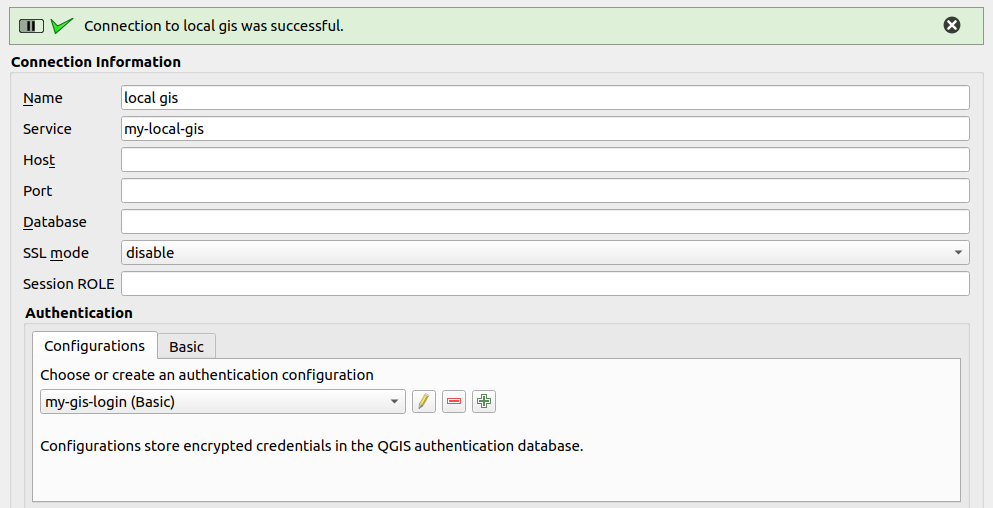
And in QGIS like this:
If you then add a layer in QGIS, only the name of the service is written in the project file. Neither the connection parameters nor username/password are saved. In addition to the security aspect, this has various advantages, more on this below.
But you don’t have to pass all of these parameters to a service. If you only pass parts of them (e.g. without the database), then you have to pass them when the connection is called:
$psql "service=my-local-gis dbname=gis"
psql (14.11 (Ubuntu 14.11-0ubuntu0.22.04.1), server 14.5 (Debian 14.5-1.pgdg110+1))
SSL connection (protocol: TLSv1.3, cipher: TLS_AES_256_GCM_SHA384, bits: 256, compression: off)
Type "help" for help.

gis=#
You can also override parameters. If you have a database gis configured in the service, but you want to connect the database web, you can specify the service and explicit the database:
$psql "service=my-local-gis dbname=web"
psql (14.11 (Ubuntu 14.11-0ubuntu0.22.04.1), server 14.5 (Debian 14.5-1.pgdg110+1))
SSL connection (protocol: TLSv1.3, cipher: TLS_AES_256_GCM_SHA384, bits: 256, compression: off)
Type "help" for help.

web=#
Of course the same applies to QGIS.
And regarding the environment variables mentioned, you can also set a standard service.
export PGSERVICE=my-local-gis
Particularly pleasant in daily work with always the same database.
$ psql
psql (14.11 (Ubuntu 14.11-0ubuntu0.22.04.1), server 14.5 (Debian 14.5-1.pgdg110+1))
SSL connection (protocol: TLSv1.3, cipher: TLS_AES_256_GCM_SHA384, bits: 256, compression: off)
Type "help" for help.

gis=#
And why is it particularly cool?
There are several reasons why such a file is useful:
Security: You don’t have to save the connection parameters anywhere in the client files (e.g. QGIS project files). Keep in mind that they are still plain text in the service file.
Decoupling: You can change the connection parameters without having to change the settings in client files (e.g. QGIS project files).
Multi-User: You can save the file on a network drive. As long as the environment variable of the local systems points to this file, all users can access the database with the same parameters.
Diversity: You can use the same project file to access different databases with the same structure if only the name of the service remains the same.
For the last reason, here are three use cases.
Support-Case
Someone reports a problem in QGIS on a specific case with their database. Since the problem cannot be reproduced, they send us a DB dump of a schema and a QGIS project file. The layers in the QGIS project file are linked to a service. Now we can restore the dump on our local database and access it with our own, but same named, service. The problem can be reproduced.
INTERLIS
With INTERLIS the structure of a database schema is precisely specified. If e.g. the canton has built the physical database for it and configured a supernice QGIS project, they can provide the project file to a company without also providing the database structure. The company can build the schema based on the INTERLIS model on its own PostgreSQL database and access it using its own service with the same name.
Test/Prod Switching
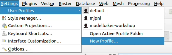
You can access a test and a production database with the same QGIS project if you have set the environment variable for the connection service file accordingly per QGIS profile.
You create two connection service files.
The one to the test database /home/dave/connectionfiles/test/pg_service.conf:
In QGIS you create two profiles “Test” and “Prod”:
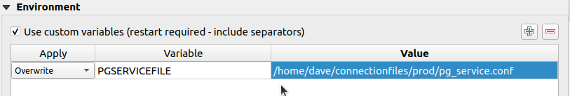
And you set the environment variable for each profile PGSERVICEFILE which should be used (in the menu Settings > Options… and there under System scroll down to Environment
or
If you now use the service my-local-gis in a QGIS layer, it connects the database prod in the “Prod” profile and the database test in the “Test” profile.
The authentication configuration
Let’s have a look at the authentication. If you have the connection service file on a network drive and make it available to several users, you may not want everyone to access it with the same login. Or you generally don’t want any user information in this file. This can be elegantly combined with the authentication configuration in QGIS.
If you want to make a QGIS project file available to multiple users, you create the layers with a service. This service contains all connection parameters except the login information.
This login information is transferred using QGIS authentication.
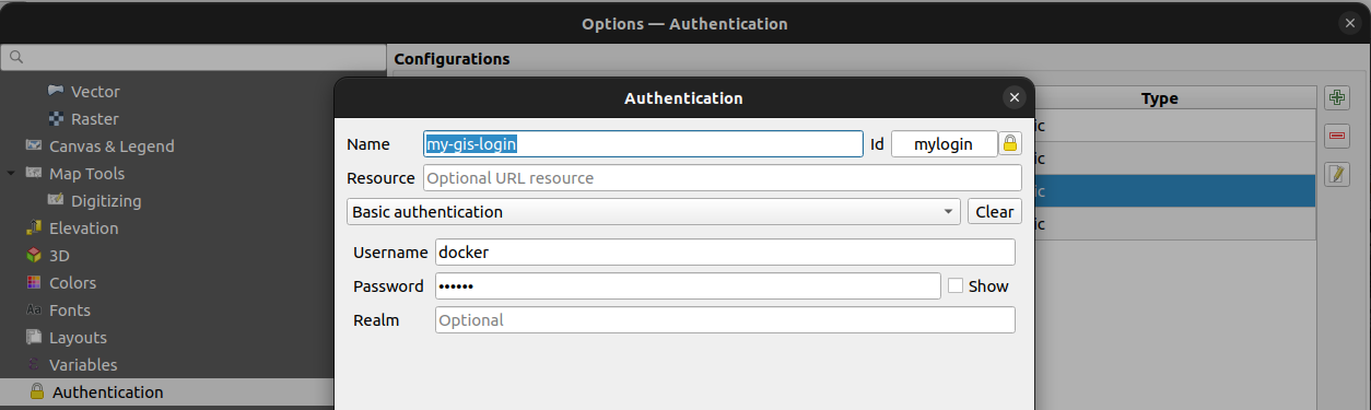
You also configure this authentication per QGIS profile we mentioned above. This is done via Menu Settings > Options… and there under Authentication:
(or directly where you create the PostgreSQL connection)
If you add such a layer, the service and the ID of the authentication configuration are saved in the QGIS project file. This is in this case mylogin. Of course this name must be communicated to the other users so that they can also set the ID for their login to mylogin.
Of course, you can use multiple authentication configurations per profile.
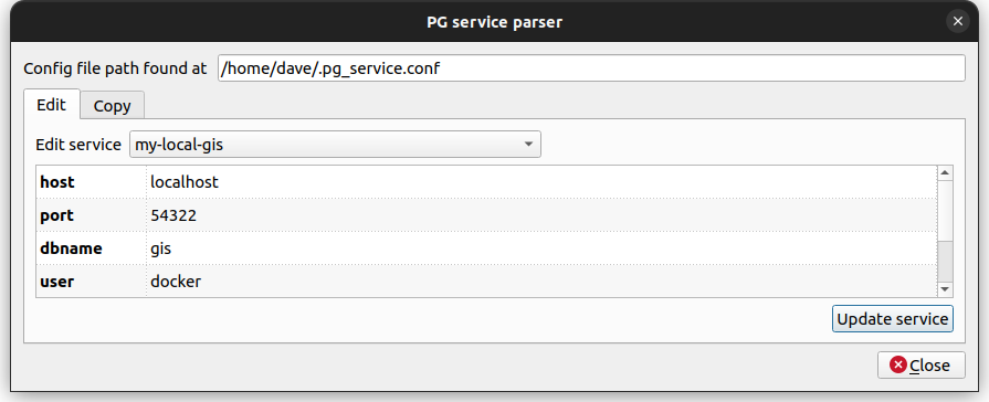
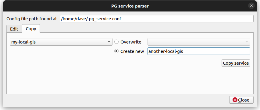
QGIS Plugin
And yes, there is now a great plugin to configure these services directly in QGIS. This means you no longer have to deal with text-based INI files. It’s called PG service parser:
It finds the connection service file according to the mentioned environment variables PGSERVICEFILE or PGSYSCONFDIR or at its default location.
As well it’s super easy to create new services by duplicating existing ones.
And for the Devs
And what would a blog post be without some geek food? The back end of this plugin is published on PYPI and can be easily installed with pip install pgserviceparser and then be used in Python.
There are some more functions. Check them out here on GitHub or in the documentation.
Well then
We hope you share our enthusiasm for this beautiful file – at least after reading this blog post. And if not – feel free to tell us why you don’t in the comments
At OPENGIS.CH, we’ve been working lately on improving the DXF Export QGIS functionality for the upcoming release 3.38. In the meantime, we’ve also added nice UX enhancements for making it easier and much more powerful to use!
Let’s see a short review.
DXF Export app dialog and processing algorithm harmonized
You can use either the app dialog or the processing algorithm, both of them offer you equivalent functionality. They are now completely harmonized!
Export settings can now be exported to an XML file
You can now have multiple settings per project available in XML, making it possible to reuse them in your workflows or share them with colleagues.
Load DXF settings from XML.
All settings are now well remembered between dialog sessions
QGIS users told us there were some dialog options that were not remembered between QGIS sessions and had to be reconfigured each time. That’s no longer the case, making it easier to reuse previous choices.
“Output layer attribute” column is now always visible in the DXF Export layer tree
We’ve made sure that you won’t miss it anymore.
Possibility to export only the current map selection
Filter features to be exported via layer selection, and even combine this filter with the existing map extent one.
Empty layers are no longer exported to DXF
When applying spatial filters like feature selection and map extent, you might end up with empty layers to be exported. Well, those won’t be exported anymore, producing cleaner DXF output files for you.
Possibility to override the export name of individual layers
It’s often the case where your layer names are not clean and tidy to be displayed. From now on, you can easily specify how your output DXF layers should be named, without altering your original project layers.
Override output layer names for DXF export.
We’ve also fixed some minor UX bugs and annoyances that were present when exporting layers to DXF format, so that we can enjoy using it. Happy DXF exporting!
We would like to thank the Swiss QGIS user group for giving us the possibility to improve the important DXF part of QGIS
Focused on stability and usability improvements, most users will find something to celebrate in QField 3.2
Main highlights
This new release introduces project-defined tracking sessions, which are automatically activated when the project is loaded. Defined while setting up and tweaking a project on QGIS, these sessions permit the automated tracking of device positions without taking any action in QField beyond opening the project itself. This liberates field users from remembering to launch a session on app launch and lowers the knowledge required to collect such data. For more details, please read the relevant QField documentation section.
As good as the above-described functionality sounds, it really shines through in cloud projects when paired with two other new featurs.
First, cloud projects can now automatically push accumulated changes at regular intervals. The functionality can be manually toggled for any cloud project by going to the synchronization panel in QField and activating the relevant toggle (see middle screenshot above). It can also be turned on project load by enabling automatic push when setting up the project in QGIS via the project properties dialog. When activated through this project setting, the functionality will always be activated, and the need for field users to take any action will be removed.
Pushing changes regularly is great, but it could easily have gotten in the way of blocking popups. This is why QField 3.2 can now push changes and synchronize cloud projects in the background. We still kept a ‘successfully pushed changes’ toast message to let you know the magic has happened
With all of the above, cloud projects on QField can now deliver near real-time tracking of devices in the field, all configured on one desktop machine and deployed through QFieldCloud. Thanks to Groupements forestiers Québec for sponsoring these enhancements.
Other noteworthy feature additions in this release include:
A brand new undo/redo mechanism allows users to rollback feature addition, editing, and/or deletion at will. The redesigned QField main menu is accessible by long pressing on the top-left dashboard button.
Support for projects’ titles and copyright map decorations as overlays on top of the map canvas in QField allows projects to better convey attributions and additional context through informative titles.
Additional improvements
The QFieldCloud user experience continues to be improved. In this release, we have reworked the visual feedback provided when downloading and synchronizing projects through the addition of a progress bar as well as additional details, such as the overall size of the files being fetched. In addition, a visual indicator has been added to the dashboard and the cloud projects list to alert users to the presence of a newer project file on the cloud for projects locally available on the device.
With that said, if you haven’t signed onto QFieldCloud yet, try it! Psst, the community account is free
The creation of relationship children during feature digitizing is now smoother as we lifted the requirement to save a parent feature before creating children. Users can now proceed in the order that feels most natural to them.
Finally, Android users will be happy to hear that a significant rework of native camera, gallery, and file picker activities has led to increased stability and much better integration with Android itself. Activities such as the gallery are now properly overlayed on top of the QField map canvas instead of showing a black screen.
The launch of QField 3.0 was a big deal, but now we’re back to focusing on smaller, more frequent updates. Don’t let the shorter change log for 3.1 trick you – there are lots of cool new features in this update!
Main highlights
One of the main improvements in this release is the brand-new functionality to enable snapping to common angles while digitizing. When enabled, the coordinate cursor will snap to configured angles alongside a visual guideline. This comes in handy when adding new geometries while surveying features with regular angles (e.g. buildings, parking lots, etc.). As QField gets more digitizing functionalities, we’ve taken the time to implement a nifty UI that collapses digitizing toggle buttons into a drawer, leaving extra space for the map canvas to shine through.
In addition, the vertex editor – one of QField’s most advanced geometry tools – received tons of love during this development cycle, focusing on improving its usability. Changes worth mentioning include:
A new undo button allows users to revert individual vertex manipulations in case of mistaken adjustment, which can save you from having to cancel a large set of ongoing manipulations;
The possibility to select vertices using finger tapping on the screen, dramatically improving the user experience;
Clearer on-screen markers to represent vertices and
Tons of bug fixes to the vertex editor itself, as well as the broader set of geometry tools.
It is now possible to lock the geometry of individual features within a single vector layer. While QField has long supported the concept of a locked geometry state for vector layers, that was until now a layer-wide toggle. With the new version of QField, a data-defined property can dictate whether a given feature geometry can be edited. Interested in geofenced geometry editing? We’ve got you covered This functionality requires the latest version of QFieldSync, which is available through QGIS’ plugin manager.
Noticeably improvements
Permission handling has been improved across all platforms. On Android, QField now delays the permission request for camera, microphone, location, and Bluetooth access until needed. This makes for a much friendlier user experience.
QField 3.0 was one of the largest releases, with major changes in its underlying libraries, including a migration to Qt 6. With the community’s help, we have spent countless hours testing before release. However, it is never a bulletproof process, and that version came with a few noticeable regressions. In particular, camera handling on Android suffered from upstream issues with Qt. We’ve tracked as many of those as possible, making this new version much more stable. One lingering camera issue remains and will be fixed upstream in the next three weeks; we’ll update as soon as it is available.
Finally, long-time users of QField will notice improvements in how geometry highlights and digitizing rubber bands are drawn. We’ve doubled down on efforts to ensure that the digitized geometries and the coordinate cursor itself are always clearly visible, whether overlaid against the canvas’s light or dark parts.
We want to extend a heartfelt thank you to our sponsors for their generous support. If you’re inspired by the developments in QField and want to contribute, please consider donating. Your support will help us continue to innovate and improve this tool for everyone’s benefit.
Shipped with many new features and built with the latest generation of Qt’s cross-platform framework, this new chapter marks an important milestone for the most powerful open-source field GIS solution.
Main highlights
Upon launching this new version of QField, users will be greeted by a revamped recent projects list featuring shiny map canvas thumbnails. While this is one of the most obvious UI improvements, countless interface tweaks and harmonization have occurred. From the refreshed dark theme to the further polishing of countless widgets, QField has never looked and felt better.
The top search bar has a new functionality that allows users to look for features within the currently active vector layer by matching any of its attributes against a given search term. Users can also refine their searches by specifying a specific attribute. The new functionality can be triggered by typing the ‘f’ prefix in the search bar followed by a string or number to retrieve a list of matching features. When expanding it, a new list of functionalities appears to help users discover all of the tools available within the search bar.
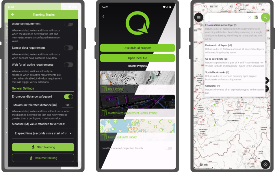
QField’s tracking has also received some love. A new erroneous distance safeguard setting has been added, which, when enabled, will dictate the tracker not to add a new vertex if the distance between it and the previously added vertex is greater than a user-specified value. This aims at preventing “spikes” of poor position readings during a tracking session. QField is now also capable of resuming a tracking session after being stopped. When resuming, tracking will reuse the last feature used when first starting, allowing sessions interrupted by battery loss or momentary pause to be continued on a single line or polygon geometry.
On the feature form front, QField has gained support for feature form text widgets, a new read-only type introduced in QGIS 3.30, which allows users to create expression-based text labels within complex feature form configurations. In addition, relationship-related form widgets now allow for zooming to children/parent features within the form itself.
To enhance digitizing work in the field, QField now makes it possible to turn snapping on and off through a new snapping button on top of the map canvas when in digitizing mode. When a project has enabled advanced snapping, the dashboard’s legend item now showcases snapping badges, allowing users to toggle snapping for individual vector layers.
QField 3.0 snapping capabilities
In addition, digitising lines and polygons by using the volume up/down hardware keys on devices such as smartphones is now possible. This can come in handy when digitizing data in harsh conditions where gloves can make it harder to use a touch screen.
While we had to play favourites in describing some of the new functionalities in QField, we’ve barely touched the surface of this feature-packed release. Other major additions include support for Near-Field Communication (NFC) text tag reading and a new geometry editor’s eraser tool to delete part of lines and polygons as you would with a pencil sketch using an eraser.
Starting with this new version, the scale bar overlay will now respect projects’ distance measurement units, allowing for scale bars in imperial and nautical units.
QField now offers a rendering quality setting which, at the cost of a slightly reduced visual quality, results in faster rendering speeds and lower memory usage. This can be a lifesaver for older devices having difficulty handling large projects and helps save battery life.
Vector tile layer support has been improved with the automated download of missing fonts and the possibility of toggling label visibility. This pair of changes makes this resolution-independent layer type much more appealing.
On iOS, layouts are now printed by QField as PDF documents instead of images. While this was the case for other platforms, it only became possible on iOS recently after work done by one of our ninjas in QGIS itself.
Many thanks to DB Fahrwgdienste for sponsoring stabilization efforts and fixes during this development cycle.
Qt 6, the latest generation of the cross-platform framework powering QField
Last but not least, QField 3.0 is now built against Qt 6. This is a significant technological milestone for the project as this means we can fully leverage the latest technological innovations into this cross-platform framework that has been powering QField since day one.
On top of the new possibilities, QField benefited from years of fixes and improvements, including better integration with Android and iOS platforms. In addition, the positioning framework in Qt 6 has been improved with awareness of the newer GNSS constellations that have emerged over the last decade.
Forest-themed release names
Forests are critical in climate regulation, biodiversity preservation, and economic sustainability. Beginning with QField 3.0 “Amazonia” and throughout the 3.X’s life cycle, we will choose forest names to underscore the importance of and advocate for global forest conservation.
As always, we hope you enjoy this new release. Happy field mapping!
A while back, one of our ninjas added a new algorithm in QGIS’ processing toolbox named ST-DBSCAN Clustering, short for spatio temporal density-based spatial clustering of applications with noise. The algorithm regroups features falling within a user-defined maximum distance and time duration values.
This post will walk you through one practical use for the algorithm: large-scale fire event analysis and visualization through remote-sensed fire detection. More specifically, we will be looking into one of the larger fire events which occurred in Canada’s Quebec province in June 2023.
Fetching and preparing FIRMS data
NASA’s Fire Information for Resource Management System (FIRMS) offers a fantastic worldwide archive of all fire detected through three spaceborne sources: MODIS C6.1 with a resolution of roughly 1 kilometer as well as VIIRS S-NPP and VIIRS NOAA-20 with a resolution of 375 meters. Each detected fire is represented by a point that sits at the center of the source’s resolution grid.
Each source will cover the whole world several times per day. Since detection is impacted by atmospheric conditions, a given pass by one source might not be able to register an ongoing fire event. It’s therefore advisable to rely on more than one source.
To look into our fire event, we have chosen the two fire detection sources with higher resolution – VIIRS S-NPP and VIIRS NOAA-20 – covering the whole month of June 2023. The datasets were downloaded from FIRMS’ archive download page.
After downloading the two separate datasets, we combined them into one merged geopackage dataset using QGIS processing toolbox’s Merge Vector Layers algorithm. The merged dataset will be used to conduct the clustering analysis.
In addition, we will use QGIS’s field calculator to create a new Date & Time field named ACQ_DATE_TIME using the following expression:
The above-pictured model outputs two datasets. The first dataset contains single-part points of detected fires with attributes from the original VIIRS products as well as a pair of new attributes: the CLUSTER_ID provides a unique cluster identifier for each point, and the CLUSTER_SIZE represents the sum of points forming each unique cluster. The second dataset contains multi-part points clusters representing fire events with four attributes: CLUSTER_ID and CLUSTER_SIZE which were discussed above as well as DATE_START and DATE_END to identify the beginning and end time of a fire event.
In our specific example, we will run the model using the merged dataset we created above as the “fire points layer” and select ACQ_DATE_TIME as the “date field”. The outputs will be saved as separate layers within a geopackage file.
Note that the maximum distance (0.025 degrees) and duration (72 hours) settings to form clusters have been set in the model itself. This can be tweaked by editing the model.
Visualizing a specific fire event progression on a map
Once the model has provided its outputs, we are ready to start visualizing a fire event on a map. In this practical example, we will focus on detected fires around latitude 53.0960 and longitude -75.3395.
Using the multi-part points dataset, we can identify two clustered events (CLUSTER_ID 109 and 1285) within the month of June 2023. To help map canvas refresh responsiveness, we can filter both of our output layers to only show features with those two cluster identifiers using the following SQL syntax: CLUSTER_ID IN (109, 1285).
To show the progression of the fire event over time, we can use a data-defined property to graduate the marker fill of the single-part points dataset along a color ramp. To do so, open the layer’s styling panel, select the simple marker symbol layer, click on the data-defined property button next to the fill color and pick the Assistant menu item.
In the assistant panel, set the source expression to the following: day(age(to_date('2023-07-01'),”ACQ_DATE_TIME”)). This will give us the number of days between a given point and an arbitrary reference date (2023-07-01 here). Set the values range from 0 to 30 and pick a color ramp of your choice.
When applying this style, the resulting map will provide a visual representation of the spread of the fire event over time.
Having identified a fire event via clustering easily allows for identification of the “starting point” of a fire by searching for the earliest fire detected amongst the thousands of points. This crucial bit of analysis can help better understand the cause of the fire, and alongside the color grading of neighboring points, its directionality as it expanded over time.
Analyzing a fire event through histogram
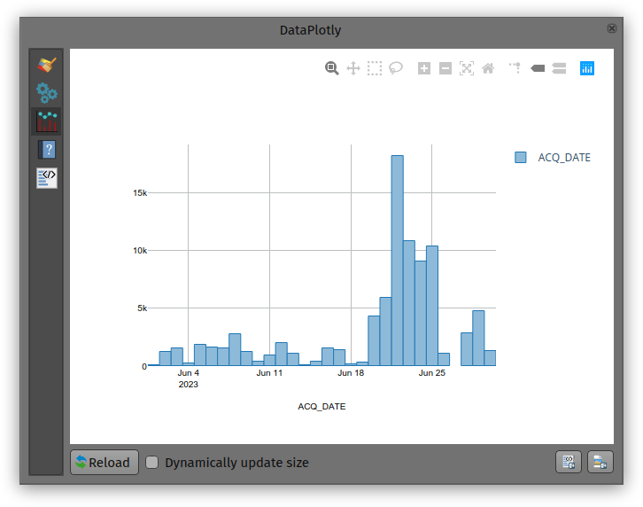
Through QGIS’ DataPlotly plugin, it is possible to create an histogram of fire events. After installing the plugin, we can open the DataPlotly panel and configure our histogram.
Set the plot type to histogram and pick the model’s single-part points dataset as the layer to gather data from. Make sure that the layer has been filtered to only show a single fire event. Then, set the X field to the following layer attribute: “ACQ_DATE”.
You can then hit the Create Plot button, go grab a coffee, and enjoy the resulting histogram which will appear after a minute or so.
While not perfect, an histogram can quickly provide a good sense of a fire event’s “peak” over a period of time.
Years ago, the QField community and its users showed their love for their favourite field app by supporting a successful crowdfunding to improve camera handling.
Since then, OPENGIS.ch has continued to lead the development of QField with the regular support of sponsors. We couldn’t be prouder of the progress we have made, with plenty of new features added in every major release. This includes major improvements to positioning including location tracking, integration of external GNSS receivers through not only Bluetooth but TCP/UDP and serial port connections, accuracy indicator and constraints, and most recently sensors reading to list a few.
We are now calling for the community to help further better QField and unlock an important milestone: background location tracking service.
Main goal: background location tracking on Android – 25’000€
Currently, QField requires users to keep their devices’ screen on and have the app in the foreground to keep track of the device’s positioning location. On mobile devices, this can drain batteries faster than many would want to, in environments where charging options are limited.
This crowdfunding aims at removing this constraint and allow QField – via a background service – to constantly keep tracking location even while the device is suspended (i.e., when the screen is turned off / locked).
To achieve this, a significant amount of work is required as the positioning framework on Android will need to be relocated to a dedicated background service. Recent work we’ve done adding a background service to synchronize captured image attachments in QFieldCloud projects armed us with the assurances that we can achieve our goal while giving us an appreciation of the large amount of work needed.
Some of the benefits
Running out of battery is the nightmare of most field surveyors. By moving location tracking to a background service, users will be able to improve their battery life considerably and keep focusing on their tasks even if it involves switching to a different app.
Furthermore, while OPENGIS.ch ninjas remain busy squashing reported QField crashes all year long, there will always be unexpected scenarios leading to abrupt app shutdowns, such as third-party apps, systems running out of battery, etc. To address this, the background service framework will also act as a safeguard to avoid location data loss when QField unexpectedly shuts down and offer users means to recover that data upon re-opening QField.
The second stretch goal builds onto QField’s nice fly-to-point navigation system. If the QField community meets this threshold, a new background navigation audio feedback informing users in the field of their proximity to their target will be implemented.
The audio feedback will use text-to-speech technology to state the distance to target in meters for a given time or distance interval.
Stretch goal 2: iOS 15’000€
The main goal will cover the Android implementation only. Due to being a very low level work we will have to replicate the work for each platform we support. If we reach stretch goal 2 we will also implement this for iOS.
Pledge now:
In case you do not see the embedded form you can open it directly here.
Thanks for supporting our crowdfunding and keep an eye on our blog for updates on the status.
Das QGIS swiss locator Plugin erleichtert in der Schweiz vielen Anwendern das Leben dadurch, dass es die umfangreichen Geodaten von swisstopo und opendata.swiss zugänglich macht. Darunter ein breites Angebot an GIS Layern, aber auch Objektinformationen und eine Ortsnamensuche.
Dank eines Förderprojektes der Anwendergruppe Schweiz durfte OPENGIS.ch ihr Plugin um eine zusätzliche Funktionalität erweitern. Dieses Mal mit der Integration von WMTS als Datenquelle, eine ziemlich coole Sache. Doch was ist eigentlich der Unterschied zwischen WMS und WMTS?
WMS vs. WMTS
Zuerst zu den Gemeinsamkeiten: Beide Protokolle – WMS und WMTS – sind dazu geeignet, Kartenbilder von einem Server zu einem Client zu übertragen. Dabei werden Rasterdaten, also Pixel, übertragen. Ausserdem werden dabei gerenderte Bilder übertragen, also keine Rohdaten. Diese sind dadurch für die Präsentation geeignet, im Browser, im Desktop GIS oder für einen PDF Export.
Der Unterschied liegt im T. Das T steht für “Tiled”, oder auf Deutsch “gekachelt”. Bei einem WMS (ohne Kachelung) können beliebige Bildausschnitte angefragt werden. Bei einem WMTS werden die Daten in einem genau vordefinierten Gitternetz — als Kacheln — ausgeliefert.
Der Hauptvorteil von WMTS liegt in dieser Standardisierung auf einem Gitternetz. Dadurch können diese Kacheln zwischengespeichert (also gecached) werden. Dies kann auf dem Server geschehen, der bereits alle Kacheln vorberechnen kann und bei einer Anfrage direkt eine Datei zurückschicken kann, ohne ein Bild neu berechnen zu müssen. Es erlaubt aber auch ein clientseitiges Caching, das heisst der Browser – oder im Fall von Swiss Locator QGIS – kann jede Kachel einfach wiederverwenden, ganz ohne den Server nochmals zu kontaktieren. Dadurch kann die Reaktionszeit enorm gesteigert werden und flott mit Applikationen gearbeitet werden.
Warum also noch WMS verwenden?
Auch das hat natürlich seine Vorteile. Der WMS kann optimierte Bilder ausliefern für genau eine Abfrage. Er kann Beispielsweise alle Beschriftungen optimal platzieren, so dass diese nicht am Kartenrand abgeschnitten sind, bei Kacheln mit den vielen Rändern ist das schwieriger. Ein WMS kann auch verschiedene abgefragte Layer mit Effekten kombinieren, Blending-Modi sind eine mächtige Möglichkeit, um visuell ansprechende Karten zu erzeugen. Weiter kann ein WMS auch in beliebigen Auflösungen arbeiten (DPI), was dazu führt, dass Schriften und Symbole auf jedem Display in einer angenehmen Grösse angezeigt werden, währenddem das Kartenbild selber scharf bleibt. Dasselbe gilt natürlich auch für einen PDF Export.
Ein WMS hat zudem auch die Eigenschaft, dass im Normalfall kein Caching geschieht. Bei einer dahinterliegenden Datenbank wird immer der aktuelle Datenstand ausgeliefert. Das kann auch gewünscht sein, zum Beispiel soll nicht zufälligerweise noch der AV-Datensatz von gestern ausgeliefert werden.
Dies bedingt jedoch immer, dass der Server das auch entsprechend umsetzt. Bei den von swisstopo via map.geo.admin.ch publizierten Karten ist die Schriftgrösse auch bei WMS fix ins Kartenbild integriert und kann nicht vom Server noch angepasst werden.
Im Falle von QGIS Swiss Locator geht es oft darum, Hintergrundkarten zu laden, z.B. Orthofotos oder Landeskarten zur Orientierung. Daneben natürlich oft auch auch weitere Daten, von eher statischer Natur. In diesem Szenario kommen die Vorteile von WMTS bestmöglich zum tragen. Und deshalb möchten wir der QGIS Anwendergruppe Schweiz im Namen von allen Schweizer QGIS Anwender dafür danken, diese Umsetzung ermöglicht zu haben!
Der QGIS Swiss Locator ist das schweizer Taschenmesser von QGIS. Fehlt dir ein Werkzeug, das du gerne integrieren würdest? Schreib uns einen Kommentar!
The latest version of QField is out, featuring as its main new feature sensor handling alongside the usual round of user experience and stability improvements. We simply can’t wait to see the sensor uses you will come up with!
The main highlight: sensors
QField 2.8 ships with out-of-the-box handling of external sensor streams over TCP, UDP, and serial port. The functionality allows for data captured through instruments – such as geiger counter, decibel sensor, CO detector, etc. – to be visualized and manipulated within QField itself.
Things get really interesting when sensor data is utilized as default values alongside positioning during the digitizing of features. You are always one tap away from adding a point locked onto your current position with spatially paired sensor readings saved as point attribute(s).
The development of this feature involved the addition of a sensor framework in upstream QGIS which will be available by the end of this coming June as part of the 3.32 release. This is a great example of the synergy between QField and its big brother QGIS, whereas development of new functionality often benefits the broader QGIS community. Big thanks to Sevenson Environmental Services for sponsoring this exciting capability.
Notable improvements
A couple of refinements during this development cycle are worth mentioning. If you ever wished for QField to directly open a selected project or reloading the last session on app launch, you’ll be happy to know this is now possible.
For heavy users of value relations in their feature forms, QField is now a tiny bit more clever when displaying string searches against long lists, placing hits that begin with the matched string first as well as visually highlighting matches within the result list itself.
Finally, feature lists throughout QField are now sorted. By default, it will sort by the display field or expression defined for each vector layer, unless an advanced sorting has been defined in a given vector layer’s attribute table. It makes browsing through lists feel that much more natural.
A brand new version of QField has been released, packed with features that will make you fall in love with this essential open source tool all over again with a focus on capturing more while you are in the field. QField 2.7 nicknamed “Heroic Hedgehog” also includes a number of worthy fixes making it a crucial update to get.
New recording capabilities
The highlight of QField 2.7 is the new audio and video recording capability straight from the feature form. In addition to preexisting still photo capture, this functionality allows for video motion and audio clips to be added as attachments to feature attributes.
The audio recording capability can come in handy in the field when typing on a keyboard-less device can be challenging. Simply record an audio note of observations to process later.
The experience wouldn’t be complete without audio and video playback support, which we took care of in this version too. Playback of such media content within the feature form gives an immediate feedback and saves time. For those interested in full screen immersion, simply click on the video frame to open the attached in your favorite media player. We also took the opportunity to implement audio and video playback on QGIS so people can easily consume the fruits of their labor in the field at their workstation.
We would be remiss if we didn’t mention map canvas rotation functionality added in this version. This is a long-requested functionality which we are happy to have packed into QField now. Pro-tip: when positioning is enabled, double tapping on the lower-left positioning button will have the map canvas follow both the device’s current location as well as the compass orientation.
Finally – some would argue “most importantly” – QField is now equipped with a beautiful dark theme which users can activate in the settings panel. By default on Android and iOS, QField will follow the system’s dark theme setting. In addition to the new color scheme, users can also adjust the user interface font size.
Big thanks to Deutsches Archäologisches Institut who funded the majority of the new features in this release cycle. Their investment in making QField the perfect tool for them has benefited the community as a whole.
A ton of bug fixing across all platforms
Important stability improvements and fixes to serious issues are also part of this release. Noteworthy fixes include WFS layer support on iOS, much better Bluetooth connectivity on Android, and vertical grid improvement on Windows.
For users facing reliability issues with the native camera on Android, we have spent time supersizing the camera we ship within QField itself. During this development cycle, it has gained zoom and flash controls, as well as a ton of usability improvements, including geo-tagging.
It’s only been a few weeks into the new year, but we’ve got great news for you: a brand new QField 2.6 “Geeky Gecko ?” has been released with a focus on positioning improvements, including Bluetooth support for Windows. And with that, we are delighted to remove the ‘beta’ status from QField for Windows.
New positioning features
Let’s open with a bang: QField 2.6 now supports NMEA streaming from external GNSS devices over TCP, UDP, and serial ports, in addition to preexisting Bluetooth connectivity. This new functionality means that QField is now compatible with a much larger range of GNSS devices out there.
These new receivers unlock NTRIP-driven centimetre accuracy for devices that use the Bluetooth connection to a manufacturer’s application to connect to NTRIP servers. In this scenario, QField could not initiate a Bluetooth connection since it was already taken. With the new TCP and UDP receivers – provided the manufacturer’s application offers NMEA streaming over either of those Internet protocols – QField can connect and consume high-accuracy positioning.
The presence of a serial port receiver provides support for external GNSS devices using Bluetooth on Windows via the virtual serial port created by the operating system. The lack of Bluetooth support on Windows was a long-wanted enhancement from QField users on that platform and was the last blocker for the ‘beta’ status to go away.
In addition, QField 2.6 allows users to pick from half a dozen metrics a value to attach to the measure (M) dimension of geometries being digitized when locked to the current position. This functionality is available to both users digitizing and the positioning tracker. The measurement values available as of 2.6 are timestamp, ground speed, bearing, horizontal accuracy and vertical accuracy, as well as PDOP, HDOP and VDOP values.
Growing Continuous Integration (CI) testing framework now covers positioning
Starting with version 2.6, QField ships with increased quality assurances thanks to the addition of tests covering positioning functionalities in its growing CI framework.
Practically speaking, this means that every single line of QField code changed is now being tested against positioning-related regression, significantly decreasing the risks of shipping a new version of QField with broken functionality in the area of antenna height, vertical grid shift, and ellipsoidal height adjustments.
We would like to commend Deutsche Bahn for funding the required work here. This could not have come in soon enough as more and more people are opting for QField and relying on it for their crucial day-to-day fieldwork.
Thanks to the sponsoring of the Swiss QGIS User Group, starting from QGIS 3.26 is it possible to override field names in the layer export dialog. Previous to that, QGIS would always export with the technical names from the database, whereas now it’s possible to override with the alias defined in QGIS or any custom name. One use for this in Switzerland — a highly polyglot country — is an export with translated names.
This is done via an additional column “Export name”. For convenience we also added a tri-state checkbox to toggle export names to their alias defined in the layer configuration or back to the field name. If a name is changed by hand the checkbox shows a mixed state.
QField is a community-driven open-source project. It is free to share, use and modify and it will stay like that. The very essence of a community is to help and support each other. And that’s where YOU come into play. To make it work we need your support!
For those who don’t know much about the concept of open source projects, a bit of background. Investing in open-source projects is a technical and ethical decision for OPENGIS.ch. Open source is a technological advantage, as we receive input from many developers worldwide who are motivated to work out the best possible software. It prevents our customers from vendor lock-in and allows complete ownership and control of the developed software. And finally, not only financially independent businesses and people should benefit from professional software but also those who might not have the financial means to pay for features, and licences.
You are not a developer, but you still like to use QField and support it? Good news. You don’t have to be a developer to use, contribute or recommend the app. There are plenty of things that need to be done to help QField to remain the powerful software it is right now and become even better. Here are a few suggestions on how you can give something back.
Let the world know about it! It doesn’t matter if you’re on Twitter, LinkedIn, Instagram or any other social media platform. Show and tell about where QField helped you. We appreciate every post and we promise to like, share and comment.
Write about your experience and please let us know. Be it in your blog or as a new success story. Insights into field projects are extremely valuable. It helps us to make the app even more efficient for your work, and it helps others to understand the range of applications for QField.
Register for a paid QFieldCloud account. QFieldCloud allows to synchronize and merge the data collected in QField. QFieldCloud is hosted by the makers of QField and by getting an account you help QField too.
Do you want to do something that is more hands-on and directly linked to the app? No problem.
Help with the documentation. You can document features, or improve the documentation in English. Read the how-to guide to get started.
Become a beta tester and be the first to report a bug! When something doesn’t work properly it might be a bug. The quicker we know about it, the faster it can be resolved.
If you are a developer and you want to get involved in QField development, please refer to the individual documentation for QField, QFieldCloud and QFieldSync.
And now finally for those of you who have the financial means, you can either sponsor a feature or subscribe to one of the monthly sponsorships. By doing so you help get freshly baked QField versions straight to everyone’s devices.
Nothing in it for you? In that case, just drop by to say thank you or have a hot or cold beverage with us next time you meet OPENGIS.ch at a conference and you might make our day! Want to know more about the idea of community-driven open-source projects and the QGIS project in particular? Check out Nyall Dawson’s blog post about how to effectively get things done in open source!


 or
or  . That’s why we’re very pleased that last week we could join the Swiss QGIS user day for the second time after the pandemic.


 ). We will also need the QFieldSync plugin in QGIS, which can be enabled through the QGIS plugin manager.