


OSM data quality assessment: producing map to illustrate data quality
At Oslandia, we like working with Open Source tool projects and handling Open (geospatial) Data. In this article series, we will play with the OpenStreetMap (OSM) map and subsequent data. Here comes the eighth article of this series, dedicated to the OSM data quality evaluation, through production of new maps.
1 Description of OSM element
1.1 Element metadata extraction
As mentionned in a previous article dedicated to metadata extraction, we have to focus on element metadata itself if we want to produce valuable information about quality. The first questions to answer here are straightforward: what is an OSM element? and how to extract its associated metadata?. This part is relatively similar to the job already done with users.
We know from previous analysis that an element is created during a changeset by a given contributor, may be modified several times by whoever, and may be deleted as well. This kind of object may be either a “node”, a “way” or a “relation”. We also know that there may be a set of different tags associated with the element. Of course the list of every operations associated to each element is recorded in the OSM data history. Let’s consider data around Bordeaux, as in previous blog posts:
import pandas as pd
elements = pd.read_table('../src/data/output-extracts/bordeaux-metropole/bordeaux-metropole-elements.csv', parse_dates=['ts'], index_col=0, sep=",")
elements.head().T
   elem        id  version  visible         ts    uid  chgset
0  node  21457126        2    False 2008-01-17  24281  653744
1  node  21457126        3    False 2008-01-17  24281  653744
2  node  21457126        4    False 2008-01-17  24281  653744
3  node  21457126        5    False 2008-01-17  24281  653744
4  node  21457126        6    False 2008-01-17  24281  653744
This short description helps us to identify some basic features, which are built in the following snippets. First we recover the temporal features:
elem_md = (elements.groupby(['elem', 'id'])['ts']
            .agg(["min", "max"])
            .reset_index())
elem_md.columns = ['elem', 'id', 'first_at', 'last_at']
elem_md['lifespan'] = (elem_md.last_at - elem_md.first_at)/pd.Timedelta('1D')
extraction_date = elements.ts.max()
elem_md['n_days_since_creation'] = ((extraction_date - elem_md.first_at)
                                  / pd.Timedelta('1d'))
elem_md['n_days_of_activity'] = (elements
                              .groupby(['elem', 'id'])['ts']
                              .nunique()
                              .reset_index())['ts']
elem_md = elem_md.sort_values(by=['first_at'])
                                    213418
elem                                  node
id                               922827508
first_at               2010-09-23 00:00:00
last_at                2010-09-23 00:00:00
lifespan                                 0
n_days_since_creation                 2341
n_days_of_activity                       1
Then the remainder of the variables, e.g. how many versions, contributors, changesets per elements:
    elem_md['version'] = (elements.groupby(['elem','id'])['version']
                          .max()
                          .reset_index())['version']
    elem_md['n_chgset'] = (elements.groupby(['elem', 'id'])['chgset']
                           .nunique()
                           .reset_index())['chgset']
    elem_md['n_user'] = (elements.groupby(['elem', 'id'])['uid']
                         .nunique()
                         .reset_index())['uid']
    osmelem_last_user = (elements
                         .groupby(['elem','id'])['uid']
                         .last()
                         .reset_index())
    osmelem_last_user = osmelem_last_user.rename(columns={'uid':'last_uid'})
    elements = pd.merge(elements, osmelem_last_user,
                       on=['elem', 'id'])
    elem_md = pd.merge(elem_md,
                       elements[['elem', 'id', 'version', 'visible', 'last_uid']],
                       on=['elem', 'id', 'version'])
    elem_md = elem_md.set_index(['elem', 'id'])
    elem_md.sample().T
elem                                  node
id                              1340445266
first_at               2011-06-26 00:00:00
last_at                2011-06-27 00:00:00
lifespan                                 1
n_days_since_creation                 2065
n_days_of_activity                       2
version                                  2
n_chgset                                 2
n_user                                   1
visible                              False
last_uid                            354363
As an illustration we have above an old two-versionned node, no more visible on the OSM website.
1.2 Characterize OSM elements with user classification
This set of features is only descriptive, we have to add more information to be able to characterize OSM data quality. That is the moment to exploit the user classification produced in the last blog post!
As a recall, we hypothesized that clustering the users permits to evaluate their trustworthiness as OSM contributors. They are either beginners, or intermediate users, or even OSM experts, according to previous classification.
Each OSM entity may have received one or more contributions by users of each group. Let’s say the entity quality is good if its last contributor is experienced. That leads us to classify the OSM entities themselves in return!
How to include this information into element metadata?
We first need to recover the results of our clustering process.
user_groups = pd.read_hdf("../src/data/output-extracts/bordeaux-metropole/bordeaux-metropole-user-kmeans.h5", "/individuals")
user_groups.head()
           PC1       PC2       PC3       PC4       PC5       PC6  Xclust
uid
1626 -0.035154  1.607427  0.399929 -0.808851 -0.152308 -0.753506       2
1399 -0.295486 -0.743364  0.149797 -1.252119  0.128276 -0.292328       0
2488  0.003268  1.073443  0.738236 -0.534716 -0.489454 -0.333533       2
5657 -0.889706  0.986024  0.442302 -1.046582 -0.118883 -0.408223       4
3980 -0.115455 -0.373598  0.906908  0.252670  0.207824 -0.575960       5
As a remark, there were several important results to save after the clustering process; we decided to serialize them into a single binary file. Pandas knows how to manage such file, that would be a pity not to take advantage of it!
We recover the individuals groups in the eponym binary file tab (column Xclust), and only have to join it to element metadata as follows:
elem_md = elem_md.join(user_groups.Xclust, on='last_uid')
elem_md = elem_md.rename(columns={'Xclust':'last_uid_group'})
elem_md.reset_index().to_csv("../src/data/output-extracts/bordeaux-metropole/bordeaux-metropole-element-metadata.csv")
elem_md.sample().T
elem                                  node
id                              1530907753
first_at               2011-12-04 00:00:00
last_at                2011-12-04 00:00:00
lifespan                                 0
n_days_since_creation                 1904
n_days_of_activity                       1
version                                  1
n_chgset                                 1
n_user                                   1
visible                               True
last_uid                             37548
last_uid_group                           2
From now, we can use the last contributor cluster as an additional information to generate maps, so as to study data quality…
Wait… There miss another information, isn’t it? Well yes, maybe the most important one, when dealing with geospatial data: the location itself!
1.3 Recover the geometry information
Even if Pyosmium library is able to retrieve OSM element geometries, we realized some tests with an other OSM data parser here: osm2pgsql.
We can recover geometries from standard OSM data with this tool, by assuming the existence of an osm database, owned by user:
osm2pgsql -E 27572 -d osm -U user -p bordeaux_metropole --hstore ../src/data/raw/bordeaux-metropole.osm.pbf
We specify a France-focused SRID (27572), and a prefix for naming output databases point, line, polygon and roads.
We can work with the line subset, that contains the physical roads, among other structures (it roughly corresponds to the OSM ways), and build an enriched version of element metadata, with geometries.
First we can create the table bordeaux_metropole_geomelements, that will contain our metadata…
DROP TABLE IF EXISTS bordeaux_metropole_elements;
DROP TABLE IF EXISTS bordeaux_metropole_geomelements;
CREATE TABLE bordeaux_metropole_elements(
       id int,
       elem varchar,
       osm_id bigint,
       first_at varchar,
       last_at varchar,
       lifespan float,
       n_days_since_creation float,
       n_days_of_activity float,
       version int,
       n_chgsets int,
       n_users int,
       visible boolean,
       last_uid int,
       last_user_group int
);
…then, populate it with the data accurate .csv file…
COPY bordeaux_metropole_elements
FROM '/home/rde/data/osm-history/output-extracts/bordeaux-metropole/bordeaux-metropole-element-metadata.csv'
WITH(FORMAT CSV, HEADER, QUOTE '"');
…and finally, merge the metadata with the data gathered with osm2pgsql, that contains geometries.
SELECT l.osm_id, h.lifespan, h.n_days_since_creation,
h.version, h.visible, h.n_users, h.n_chgsets,
h.last_user_group, l.way AS geom
INTO bordeaux_metropole_geomelements
FROM bordeaux_metropole_elements as h
INNER JOIN bordeaux_metropole_line as l
ON h.osm_id = l.osm_id AND h.version = l.osm_version
WHERE l.highway IS NOT NULL AND h.elem = 'way'
ORDER BY l.osm_id;
Wow, this is wonderful, we have everything we need in order to produce new maps, so let’s do it!
2 Keep it visual, man!
From the last developments and some hypothesis about element quality, we are able to produce some customized maps. If each OSM entities (e.g. roads) can be characterized, then we can draw quality maps by highlighting the most trustworthy entities, as well as those with which we have to stay cautious.
In this post we will continue to focus on roads within the Bordeaux area. The different maps will be produced with the help of Qgis.
2.1 First step: simple metadata plotting
As a first insight on OSM elements, we can plot each OSM ways regarding simple features like the number of users who have contributed, the number of version or the element anteriority.
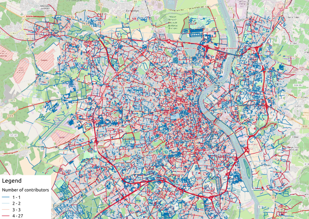
Figure 1: Number of active contributors per OSM way in Bordeaux
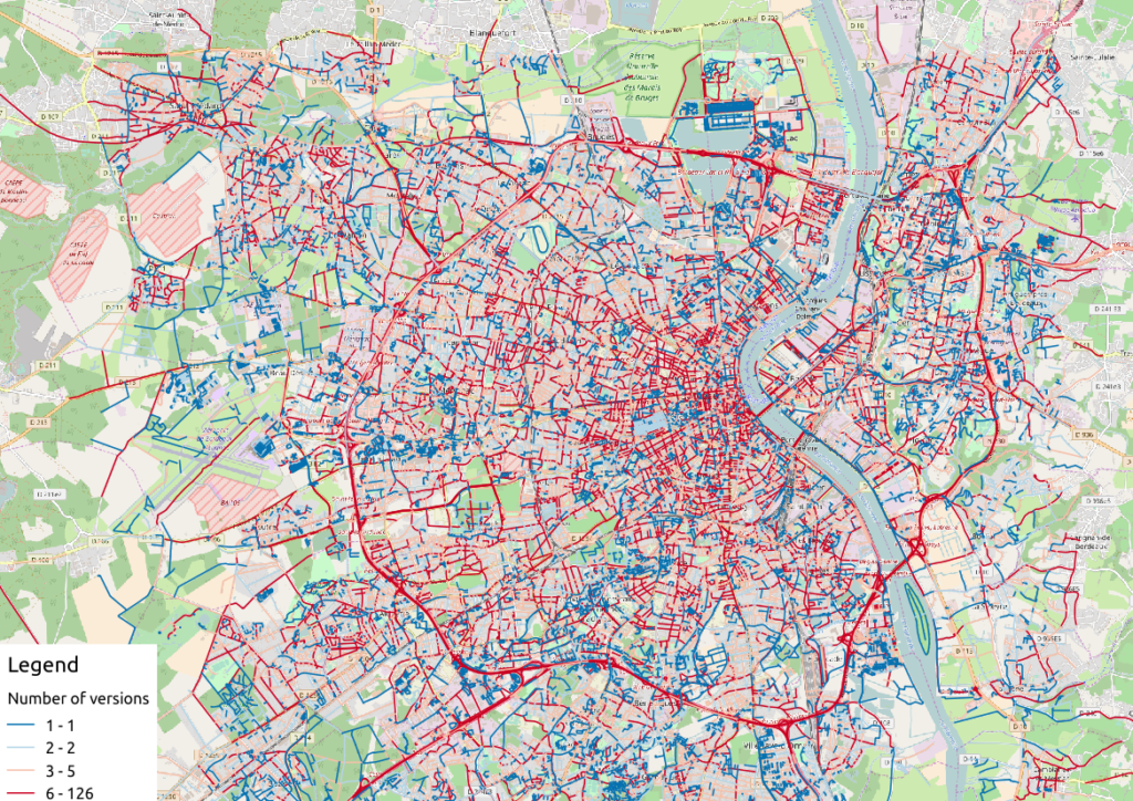
Figure 2: Number of versions per OSM way in Bordeaux
With the first two maps, we see that the ring around Bordeaux is the most intensively modified part of the road network: more unique contributors are implied in the way completion, and more versions are designed for each element. Some major roads within the city center present the same characteristics.

Figure 3: Anteriority of each OSM way in Bordeaux, in years
If we consider the anteriority of OSM roads, we have a different but interesting insight of the area. The oldest roads are mainly located within the city center, even if there are some exceptions. It is also interesting to notice that some spatial patterns arise with temporality: entire neighborhoods are mapped within the same anteriority.
2.2 More complex: OSM data merging with alternative geospatial representations
To go deeper into the mapping analysis, we can use the INSEE carroyed data, that divides France into 200-meter squared tiles. As a corollary OSM element statistics may be aggregated into each tile, to produce additional maps. Unfortunately an information loss will occur, as such tiles are only defined where people lives. However it can provides an interesting alternative illustration.
To exploit such new data set, we have to merge the previous table with the accurate INSEE table. Creating indexes on them is of great interest before running such a merging operation:
CREATE INDEX insee_geom_gist
ON open_data.insee_200_carreau USING GIST(wkb_geometry);
CREATE INDEX osm_geom_gist
ON bordeaux_metropole_geomelements USING GIST(geom);

DROP TABLE IF EXISTS bordeaux_metropole_carroyed_ways;
CREATE TABLE bordeaux_metropole_carroyed_ways AS (
SELECT insee.ogc_fid, count(*) AS nb_ways,
avg(bm.version) AS avg_version, avg(bm.lifespan) AS avg_lifespan,
avg(bm.n_days_since_creation) AS avg_anteriority,
avg(bm.n_users) AS avg_n_users, avg(bm.n_chgsets) AS avg_n_chgsets,
insee.wkb_geometry AS geom
FROM open_data.insee_200_carreau AS insee
JOIN bordeaux_metropole_geomelements AS bm
ON ST_Intersects(insee.wkb_geometry, bm.geom)
GROUP BY insee.ogc_fid
);
As a consequence, we get only 5468 individuals (tiles), a quantity that must be compared to the 29427 roads previously handled… This operation will also simplify the map analysis!
We can propose another version of previous maps by using Qgis, let’s consider the average number of contributors per OSM roads, for each tile:
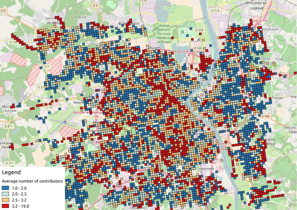
Figure 4: Number of contributors per OSM roads, aggregated by INSEE tile
2.3 The cherry on the cake: representation of OSM elements with respect to quality
Last but not least, the information about last user cluster can shed some light on OSM data quality: by plotting each roads according to the last user who has contributed, we might identify questionable OSM elements!
We simply have to design similar map than in previous section, with user classification information:
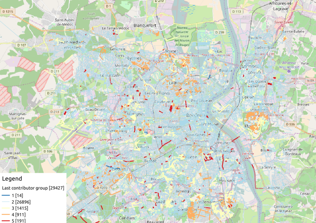
Figure 5: OSM roads around Bordeaux, according to the last user cluster (1: C1, relation experts; 2: C0, versatile expert contributors; 3: C4, recent one-shot way contributors; 4: C3, old one-shot way contributors; 5: C5, locally-unexperienced way specialists)
According to the clustering done in the previous article (be careful, the legend is not the same here…), we can make some additional hypothesis:
- Light-blue roads are OK, they correspond to the most trustful cluster of contributors (91.4% of roads in this example)
- There is no group-0 road (group 0 corresponds to cluster C2 in the previous article)… And that’s comforting! It seems that “untrustworthy” users do not contribute to roads or -more probably- that their contributions are quickly amended.
- Other contributions are made by intermediate users: a finer analysis should be undertaken to decide if the corresponding elements are valid. For now, we can consider everything is OK, even if local patterns seem strong. Areas of interest should be verified (they are not necessarily of low quality!)
For sure, it gives a fairly new picture of OSM data quality!
3 Conclusion
In this last article, we have designed new maps on a small area, starting from element metadata. You have seen the conclusion of our analysis: characterizing the OSM data quality starting from the user contribution history.
Of course some works still have to be done, however we detailed a whole methodology to tackle the problem. We hope you will be able to reproduce it, and to design your own maps!
Feel free to contact us if you are interested in this topic!
Computing network centers
How do you objectively define and compute which parts of a network are in the center? One approach is to use the concept of centrality.
Centrality refers to indicators which identify the most important vertices within a graph. Applications include identifying the most influential person(s) in a social network, key infrastructure nodes in the Internet or urban networks, and super spreaders of disease. (Source: http://en.wikipedia.org/wiki/Centrality)
Researching this topic, it turns out that some centrality measures have already been implemented in GRASS GIS. thumbs up!
v.net.centrality computes degree, betweeness, closeness and eigenvector centrality.
As a test, I’ve loaded the OSM street network of Vienna and run
v.net.centrality -a input=streets@anita_000 output=centrality degree=degree closeness=closeness betweenness=betweenness eigenvector=eigenvector

The computations take a while.
In my opinion, the most interesting centrality measures for this street network are closeness and betweenness:
Closeness “measures to which extent a node i is near to all the other nodes along the shortest paths”. Closeness values are lowest in the center of the network and higher in the outskirts.
Betweenness “is based on the idea that a node is central if it lies between many other nodes, in the sense that it is traversed by many of the shortest paths connecting couples of nodes.” Betweenness values are highest on bridges and other important arterials while they are lowest for dead-end streets.
(Definitions as described in more detail in Crucitti, Paolo, Vito Latora, and Sergio Porta. “Centrality measures in spatial networks of urban streets.” Physical Review E 73.3 (2006): 036125.)

Centrality: low values in pink, high values in green
Works great! Unfortunately, v.net.centrality is not yet part of the QGIS Processing GRASS toolbox. It would certainly be a great addition.

OSM Toner style town labels explained
The point table of the Spatialite database created from OSM north-eastern Austria contains more than 500,000 points. This post shows how the style works which – when applied to the point layer – wil make sure that only towns and (when zoomed in) villages will be marked and labeled.

In the attribute table, we can see that there are two tags which provide context for populated places: the place and the population tag. The place tag has it’s own column created by ogr2ogr when converting from OSM to Spatialite. The population tag on the other hand is listed in the other_tags column.

for example
"opengeodb:lat"=>"47.5000237","opengeodb:lon"=>"16.0334769","population"=>"623"
Overview maps would be much too crowded if we simply labeled all cities and towns. Therefore, it is necessary to filter towns based on their population and only label the bigger ones. I used limits of 5,000 and 10,000 inhabitants depending on the scale.

At the core of these rules is an expression which extracts the population value from the other_tags attribute: The strpos() function is used to locate the text "population"=>" within the string attribute value. The population value is then extracted using the left() function to get the characters between "population"=>" and the next occurrence of ". This value can ten be cast to integer using toint() and then compared to the population limit:
5000 < toint(
   left (
      substr(
         "other_tags",
         strpos("other_tags" ,'"population"=>"')+16,
         8
      ),
      strpos(
         substr(
            "other_tags",
            strpos("other_tags" ,'"population"=>"')+16,
            8
         ),
        '"'
      )
   )
)
There is also one additional detail concerning label placement in this style: When zoomed in closer than 1:400,000 the labels are placed on top of the points but when zoomed out further, the labels are put right of the point symbol. This is controlled using a scale-based expression in the label placement:

As usual, you can find the style on Github: https://github.com/anitagraser/QGIS-resources/blob/master/qgis2/osm_spatialite/osm_spatialite_tonerlite_point.qml

Will the sun shine on us?
Table Of Content
1. Creating the direct sunlight maps
2. Time to look at some details: So, is Malga Brigolina in sunlight at lunch time?
Recently, in order to nicely plan ahead for a birthday lunch at the agritur Malga Brigolina (a farm-restaurant near Sopramonte di Trento, Italy, at 1,000m a.s.l. in the Southern Alps), friends of mine asked me the day before:
“Will the place be sunny at lunch time for a nice walk?“
[well, the weather was close to clear sky conditions but mountains are high here and casting long shadows in the winter time].

A rather easy task I thought, so I got my tools ready since that was an occasion to verify the predictions with some photos! Thanks to the new EU-DEM at 25m I was able to perform the computations right away in a metric system rather than dealing with degree in LatLong.
Direct sunlight can be assessed from the beam radiation map of GRASS GIS’ r.sun when running it for a specific day and time. But even easier, there is a new Addon for GRASS GIS 7 which calculates right away time series of insolation maps given start/stop timestamps and a time step: r.sun.hourly. This shrinks the overall effort to almost nothing.
1. Creating the direct sunlight maps
The first step is to calculate where direct sunlight reaches the ground. Here the input elevation map is the European “eu_dem_25″, while the output is the beam radiation for a certain day (15 Dec 2013 is DOY 349).
Important hint: the computational region must be large enough to east/south/west to capure the cast shadow effects of all relevant surrounding mountains.
I let calculations start at 8am and finish at 5pm which an hourly time step. The authors have kindly parallelized r.sun.hourly, so I let it run on four processors simultaneously to speed up:
# calculate DOY (day-of-year) from given date:
date -d 2013-12-15 +%j
349

# calculate beam radiation maps for a given time period
# (note: minutes are to be given in decimal time: 30min = 0.5)
r.sun.hourly elev_in=eu_dem_25 beam_rad=trento_beam_doy349 \
      start_time=8 end_time=17 time_step=1 day=349 year=2013 \
      nprocs=4
The ten resulting maps contain the beam radiation for each pixel considering the cast shadow effects of the pixel-surrounding mountains. However, the question was not to calculate irradiance raster maps in Wh/m^2 but simply “sun-yes” or “sun-no”. So a subsequent filtering had to be applied. Each beam radiation map was filtered: if pixel value equal to 0 then “sun-no”, otherwise “sun-yes” (what my friends wanted to achieve; effectively a conversion into a binary map).
Best done in a simple shell script loop:
[Edit 30 Dec 2013: thanks to Anna you can simplify below loop to the r.colors call thanks to the new -b flag for binary output in r.sun.hourly!]
for map in `g.mlist rast pattern="trento_beam_doy349*"` ; do
    # rename current map to tmp
    g.rename rast=$map,$map.tmp
    # filter and save with original name
    r.mapcalc "$map = if($map.tmp == 0, null(), 1)"
    # colorize the binary map
    echo "1 yellow" | r.colors $map rules=-
    # remove cruft
    g.remove rast=$map.tmp
done
As a result we got ten binary maps, ideal for using them as overlay with shaded DEMs or OpenStreetMap layers. The areas exposed to direct sunlight are shown in yellow.

Trento, direct sunlight, 15 Dec 2013 between 10am and 5pm (See here for creating an animated GIF). Quality reduced for this blog.
2. Time to look at some details: So, is Malga Brigolina in sunlight at lunch time?
Situation at 12pm (noon): predicted that the restaurant is still in shadow – confirmed in the photo:

(click to enlarge)
Situation at 1:30/2:00pm: sun is getting closer to the Malga, as confirmed in photo (note that the left photo is 20min ahead of the map). The small street in the right photo is still in the shadow as predicted in the map):
 (click to enlarge)
Situation at 3:00pm: sun here and there at Malga Brigolina:
 Sunlight map blended with OpenStreetmap layer (r.blend + r.composite) and draped over DEM in wxNVIZ of GRASS GIS 7 (click to enlarge). The sunday walk path around Malga Brigolina is the blue/red vector line shown in the view center.
Situation at 4:00pm: we are close to sunset in Trentino… view towards the Rotaliana (Mezzocorona, S. Michele all’Adige), last sunlit summits also seen in photo:
 (click to enlarge)
3. Outcome
The resulting sunlight/shadow map appear to match nicely realty. Perhaps r.sun.hourly should get an additional flag to generate the binary “sun-yes” – “sun-no” maps directly.
 Direct sunlight zones (yellow, 15 Dec 2013, 3pm): Trento with Monte Bondone, Paganella, Marzolan, Lago di Caldonazzo, Lago di Levico and surroundings (click to enlarge)
4. GRASS GIS usage note
The wxGUI settings were as simple as this (note the transparency values for the various layers):

Data sources:
- Shaded maps produced using Copernicus data and information funded by the European Union – EU-DEM layers
- © OpenStreetMap contributors
The post Will the sun shine on us? appeared first on GFOSS Blog | GRASS GIS Courses.
Using the 25m EU-DEM for shading OpenStreetMap layers
Inspired by Václav Petráš posting about “Did you know that you can see streets of downtown Raleigh in elevation data from NC sample dataset?” I wanted to try the new GRASS GIS 7 Addon r.shaded.pca which creates shades from various directions and combines then into RGB composites just to see what happens when using the new EU-DEM at 25m.
To warm up, I registered the “normally” shaded DEM (previously generated with gdaldem) with r.external in a GRASS GIS 7 location (EPSG 3035, LAEA) and overlayed the OpenStreetMap layer using WMS with GRASS 7′s r.in.wms. An easy task thanks to University of Heidelberg’s www.osm-wms.de. Indeed, they offer a similar shading via WMS, however, in the screenshot below you see the new EU data being used for controlling the light on our own:

OpenStreetMap shaded with EU DEM 25m (click to enlarge)
Next item: trying r.shaded.pca… It supports multi-core calculation and the possibility to strengthen the effects through z-rescaling. In my example, I used:
r.shaded.pca input=eu_dem_25 output=eu_dem_25_shaded_pca nproc=3 zmult=50
The leads to a colorized hillshading map, again with the OSM data on top (50% transparency):

OpenStreetMap shaded with r.shaded.pca using EU DEM 25m (click to enlarge)
Yes, fun – I like it ![]()
Data sources:
- Shaded maps produced using Copernicus data and information funded by the European Union – EU-DEM layers
- © OpenStreetMap contributors
The post Using the 25m EU-DEM for shading OpenStreetMap layers appeared first on GFOSS Blog | GRASS GIS Courses.
50th ICA-OSGeo Lab established at Fondazione Edmund Mach (FEM)
We are pleased to announce that the 50th ICA-OSGeo Lab has been established at the GIS and Remote Sensing Unit (Piattaforma GIS & Remote Sensing, PGIS), Research and Innovation Centre (CRI), Fondazione Edmund Mach (FEM), Italy. CRI is a multifaceted research organization established in 2008 under the umbrella of FEM, a private research foundation funded by the government of Autonomous Province of Trento. CRI focuses on studies and innovations in the fields of agriculture, nutrition, and environment, with the aim to generate new sharing knowledge and to contribute to economic growth, social development and the overall improvement of quality of life. 
The mission of the PGIS unit is to develop and provide multi-scale approaches for the description of 2-, 3- and 4-dimensional biological systems and processes. Core activities of the unit include acquisition, processing and validation of geo-physical, ecological and spatial datasets collected within various research projects and monitoring activities, along with advanced scientific analysis and data management. These studies involve multi-decadal change analysis of various ecological and physical parameters from continental to landscape level using satellite imagery and other climatic layers. The lab focuses on the geostatistical analysis of such information layers, the creation and processing of indicators, and the production of ecological, landscape genetics, eco-epidemiological and physiological models. The team pursues actively the development of innovative methods and their implementation in a GIS framework including the time series analysis of proximal and remote sensing data.
The GIS and Remote Sensing Unit (PGIS) members strongly support the peer reviewed approach of Free and Open Source software development which is perfectly in line with academic research. PGIS contributes extensively to the open source software development in geospatial (main contributors to GRASS GIS), often collaborating with various other developers and researchers around the globe. In the new ICA-OSGeo lab at FEM international PhD students, university students and trainees are present.
PGIS is focused on knowledge dissemination of open source tools through a series of courses designed for specific user requirement (schools, universities, research institutes), blogs, workshops and conferences. Their recent publication in Trends in Ecology and Evolution underlines the need on using Free and Open Source Software (FOSS) for completely open science. Dr. Markus Neteler, who is leading the group since its formation, has two decades of experience in developing and promoting open source GIS software. Being founding member of the Open Source Geospatial Foundation (OSGeo.org, USA), he served on its board of directors from 2006-2011. Luca Delucchi, focal point and responsible person for the new ICA-OSGeo Lab is member of the board of directors of the Associazione Italiana per l’Informazione Geografica Libera (GFOSS.it, the Italian Local Chapter of OSGeo). He contributes to several Free and Open Source software and open data projects as developer and trainer.
Details about the GIS and Remote Sensing Unit at http://gis.cri.fmach.it/
Open Source Geospatial Foundation (OSGeo) is a not-for-profit organisation founded in 2006 whose mission is to support and promote the collaborative development of open source geospatial technologies and data.
International Cartographic Association (ICA) is the world authoritative body for cartography and GIScience. See also the new ICA-OSGeo Labs website.
OSM Reporter Update for Open Data Day 2013
Today is Open Data Day 2013. I did’t have much time to hack, but I made a few tweaks to my ‘just for fun’ osm-reporter project to provide average, min and max counts per active day for each user. I also did a bunch of code cleanups under the hood which probably nobody except me... Read more »
User history added to osm-reporter app
This weekend I implemented a new feature for my ‘just for fun’ project osm-reporter. The feature implements timeline reporting for Open Street Map contributors. Its probably easiest to explain with a screenshot: Here is another one showing a few charts together: I added the feature because I wanted to see how many... Read more »
User history added to osm-reporter app
This weekend I implemented a new feature for my 'just for fun' project osm-reporter. The feature implements timeline reporting for Open Street Map contributors. Its probably easiest to explain with a screenshot:

Here is another one showing a few charts together:
I added the feature because I wanted to see how many person days were involved in data gathering for a particular area and feature type. It does have some limitations - it ignores deletion and ownership transfer of features. It does however provide a nice quick overview of effort. Try it on your own neighbourhood and see how much work went into the OSM coverage for your area!
I've also had some really awesome contributions from Yohan Bonifiace (added leaflet support, feature type switching, extent urls) and Sun Ning (added heatmap support). Its really great making a small, simple and limited scope project and seeing it grow with random hacks of kindness from strangers! Here is a little screenshot of the heatmap feature:

I hope you all enjoy the new version, and look forward to more improvements and suggestions from the community. Its all freely available from my github repository. You can test out the current version of the software by visiting http://osm.linfiniti.com.
OSM Building Count Stats
Here is a little update to my last post. I quickly whipped up a web app for the little stats script I wrote. It is available at http://osm.linfiniti.com. The stats only update once per hour so as not to hammer the osm export server. The code is all open source (https://github.com/timlinux/osm-reporter), written in python and... Read more »
Holiday OpenStreetMap project for Swellendam
If you even visited my lovely home town of Swellendam in the Western Cape of South Africa onhttp://openstreetmap.org, you might have noticed that the building footprints for the town are almost non-existent. Building footprints provide a valuable way to understand impacts of flood and other natural hazards, as well as being a valuable source of context information when browsing the town map. It's Christmas holiday season here in South Africa, schools have finished exams and students have time on their hands.
This year Linfiniti Consulting is sponsoring 3 students (from left to right: Jaocoline, Barbara and Nico in the image below) to capture all of the building footprints in Swellendam. Of course I was inspired by seeing the awesome work done by AIFDR, GFDRR, ACCESS and BNPB and the HOT team in Indonesia.

As well as building footprints they will also capture the building:levels and building:walls attributes so that we can in the future create a nice 3D extruded model of the towns buildings. The students are new to the OpenStreetMap project and have a lot to learn about capturing data fast and accurately, so it should be a great holiday challenge for them!
If you want to grab the current dataset for the area they are going to be working on, you can get it here (in osm format). I wrote a quick and dirty script to get the osm dump from our area and calculate how many ways each person has captured. The script is a simple python flask app. I will probably flesh it out a little as time goes by to make some pretty graphs and reports. In the mean time it just produces something like this:
JPM : 3
Firefishy : 114
uip : 1
CorliJ : 1
thomasF : 11
Chalky White : 1
Burger : 137
Sumarie : 5
Jacoline : 188
timlinux : 28
Tromilemi : 2
1st European State of the Map Conference in Vienna
The 1st European State of the Map Conference (SotM-Europe) will be held July 15-17 in Vienna, Austria. So far, there have been 4 International State of the Map conferences. This will be the first European edition of this event.
Topics include:
- Mapping (mapping, data, tagging, the state of the map in your country, etc…)
- TechTalks (development, rendering and infrastructure)
- Powered by OpenStreetMap (projects/business ideas based on OpenStreetMap)
- Convergence (open geo data world vs. the world of proprietary and authoritive data and software)
- Research (for researchers working with OpenStreetMap data)
- Others (other interesting information)
The call for papers is still open until Monday, February 28 2011.
The international conference will be held in Denver, Colorado from September 9-11 2011.


