Related Plugins and Tags

QGIS Planet

Visualization of borehole logs with QGIS

At Oslandia, we have been working on a component based on the QGIS API for the visualization of well and borehole logs.

This component is aiming at displaying data collected vertically along wells dug underground. It mainly focuses on data organized in series of contiguous samples, and is generic enough to be used for both vertical (where the Y axis corresponds to a depth underground) and horizontal data (where the X axis corresponds to time for example). One of the main concerns was to ensure good display performances with an important volume of sample points (usually hundred of thousands sample points).

We have already been working on plot components in the past, but for specific QGIS plugins (both for timeseries and stratigraphic logs) and thought we will put these past experiences to good use by creating a more generic library.

We decided to represent sample points as geometry features in order to be able to reuse the rich symbology engine of QGIS. This allows users to represent their data whatever they like without having to rewrite an entire symbology engine. We also benefit from all the performance optimizations that have been added and polished over the years (on-the-fly geometry simplification for example).

Albeit written in Python, we achieved good display performances. The key trick was to avoid copy of data between the sample points read by QGIS and the Python graphing component. It is achieved thanks to the fact that the PyQGIS API has some functions that respect the buffer protocol.

You can have a look at the following video to see this component integrated in an existing plugin.

Visualization of borehole logs withing QGIS

It is distributed as usual under an open source license and the code repository can be found on GitHub.

Do not hesitate to contact us ( [email protected] ) if you are interested in any enhancements around this component.

OSM data quality assessment: producing map to illustrate data quality

At Oslandia, we like working with Open Source tool projects and handling Open (geospatial) Data. In this article series, we will play with the OpenStreetMap (OSM) map and subsequent data. Here comes the eighth article of this series, dedicated to the OSM data quality evaluation, through production of new maps.

1 Description of OSM element

 1.1 Element metadata extraction

As mentionned in a previous article dedicated to metadata extraction, we have to focus on element metadata itself if we want to produce valuable information about quality. The first questions to answer here are straightforward: what is an OSM element? and how to extract its associated metadata?. This part is relatively similar to the job already done with users.

We know from previous analysis that an element is created during a changeset by a given contributor, may be modified several times by whoever, and may be deleted as well. This kind of object may be either a “node”, a “way” or a “relation”. We also know that there may be a set of different tags associated with the element. Of course the list of every operations associated to each element is recorded in the OSM data history. Let’s consider data around Bordeaux, as in previous blog posts:

import pandas as pd
elements = pd.read_table('../src/data/output-extracts/bordeaux-metropole/bordeaux-metropole-elements.csv', parse_dates=['ts'], index_col=0, sep=",")
elements.head().T
   elem        id  version  visible         ts    uid  chgset
0  node  21457126        2    False 2008-01-17  24281  653744
1  node  21457126        3    False 2008-01-17  24281  653744
2  node  21457126        4    False 2008-01-17  24281  653744
3  node  21457126        5    False 2008-01-17  24281  653744
4  node  21457126        6    False 2008-01-17  24281  653744

This short description helps us to identify some basic features, which are built in the following snippets. First we recover the temporal features:

elem_md = (elements.groupby(['elem', 'id'])['ts']
            .agg(["min", "max"])
            .reset_index())
elem_md.columns = ['elem', 'id', 'first_at', 'last_at']
elem_md['lifespan'] = (elem_md.last_at - elem_md.first_at)/pd.Timedelta('1D')
extraction_date = elements.ts.max()
elem_md['n_days_since_creation'] = ((extraction_date - elem_md.first_at)
                                  / pd.Timedelta('1d'))
elem_md['n_days_of_activity'] = (elements
                              .groupby(['elem', 'id'])['ts']
                              .nunique()
                              .reset_index())['ts']
elem_md = elem_md.sort_values(by=['first_at'])
                                    213418
elem                                  node
id                               922827508
first_at               2010-09-23 00:00:00
last_at                2010-09-23 00:00:00
lifespan                                 0
n_days_since_creation                 2341
n_days_of_activity                       1

Then the remainder of the variables, e.g. how many versions, contributors, changesets per elements:

    elem_md['version'] = (elements.groupby(['elem','id'])['version']
                          .max()
                          .reset_index())['version']
    elem_md['n_chgset'] = (elements.groupby(['elem', 'id'])['chgset']
                           .nunique()
                           .reset_index())['chgset']
    elem_md['n_user'] = (elements.groupby(['elem', 'id'])['uid']
                         .nunique()
                         .reset_index())['uid']
    osmelem_last_user = (elements
                         .groupby(['elem','id'])['uid']
                         .last()
                         .reset_index())
    osmelem_last_user = osmelem_last_user.rename(columns={'uid':'last_uid'})
    elements = pd.merge(elements, osmelem_last_user,
                       on=['elem', 'id'])
    elem_md = pd.merge(elem_md,
                       elements[['elem', 'id', 'version', 'visible', 'last_uid']],
                       on=['elem', 'id', 'version'])
    elem_md = elem_md.set_index(['elem', 'id'])
    elem_md.sample().T
elem                                  node
id                              1340445266
first_at               2011-06-26 00:00:00
last_at                2011-06-27 00:00:00
lifespan                                 1
n_days_since_creation                 2065
n_days_of_activity                       2
version                                  2
n_chgset                                 2
n_user                                   1
visible                              False
last_uid                            354363

As an illustration we have above an old two-versionned node, no more visible on the OSM website.

1.2 Characterize OSM elements with user classification

This set of features is only descriptive, we have to add more information to be able to characterize OSM data quality. That is the moment to exploit the user classification produced in the last blog post!

As a recall, we hypothesized that clustering the users permits to evaluate their trustworthiness as OSM contributors. They are either beginners, or intermediate users, or even OSM experts, according to previous classification.

Each OSM entity may have received one or more contributions by users of each group. Let’s say the entity quality is good if its last contributor is experienced. That leads us to classify the OSM entities themselves in return!

How to include this information into element metadata?

We first need to recover the results of our clustering process.

user_groups = pd.read_hdf("../src/data/output-extracts/bordeaux-metropole/bordeaux-metropole-user-kmeans.h5", "/individuals")
user_groups.head()
           PC1       PC2       PC3       PC4       PC5       PC6  Xclust
uid                                                                     
1626 -0.035154  1.607427  0.399929 -0.808851 -0.152308 -0.753506       2
1399 -0.295486 -0.743364  0.149797 -1.252119  0.128276 -0.292328       0
2488  0.003268  1.073443  0.738236 -0.534716 -0.489454 -0.333533       2
5657 -0.889706  0.986024  0.442302 -1.046582 -0.118883 -0.408223       4
3980 -0.115455 -0.373598  0.906908  0.252670  0.207824 -0.575960       5

As a remark, there were several important results to save after the clustering process; we decided to serialize them into a single binary file. Pandas knows how to manage such file, that would be a pity not to take advantage of it!

We recover the individuals groups in the eponym binary file tab (column Xclust), and only have to join it to element metadata as follows:

elem_md = elem_md.join(user_groups.Xclust, on='last_uid')
elem_md = elem_md.rename(columns={'Xclust':'last_uid_group'})
elem_md.reset_index().to_csv("../src/data/output-extracts/bordeaux-metropole/bordeaux-metropole-element-metadata.csv")
elem_md.sample().T
elem                                  node
id                              1530907753
first_at               2011-12-04 00:00:00
last_at                2011-12-04 00:00:00
lifespan                                 0
n_days_since_creation                 1904
n_days_of_activity                       1
version                                  1
n_chgset                                 1
n_user                                   1
visible                               True
last_uid                             37548
last_uid_group                           2

From now, we can use the last contributor cluster as an additional information to generate maps, so as to study data quality…

Wait… There miss another information, isn’t it? Well yes, maybe the most important one, when dealing with geospatial data: the location itself!

1.3 Recover the geometry information

Even if Pyosmium library is able to retrieve OSM element geometries, we realized some tests with an other OSM data parser here: osm2pgsql.

We can recover geometries from standard OSM data with this tool, by assuming the existence of an osm database, owned by user:

osm2pgsql -E 27572 -d osm -U user -p bordeaux_metropole --hstore ../src/data/raw/bordeaux-metropole.osm.pbf

We specify a France-focused SRID (27572), and a prefix for naming output databases point, line, polygon and roads.

We can work with the line subset, that contains the physical roads, among other structures (it roughly corresponds to the OSM ways), and build an enriched version of element metadata, with geometries.

First we can create the table bordeaux_metropole_geomelements, that will contain our metadata…

DROP TABLE IF EXISTS bordeaux_metropole_elements;
DROP TABLE IF EXISTS bordeaux_metropole_geomelements;
CREATE TABLE bordeaux_metropole_elements(
       id int,
       elem varchar,
       osm_id bigint,
       first_at varchar,
       last_at varchar,
       lifespan float,
       n_days_since_creation float,
       n_days_of_activity float,
       version int,
       n_chgsets int,
       n_users int,
       visible boolean,
       last_uid int,
       last_user_group int
);

…then, populate it with the data accurate .csv file…

COPY bordeaux_metropole_elements
FROM '/home/rde/data/osm-history/output-extracts/bordeaux-metropole/bordeaux-metropole-element-metadata.csv'
WITH(FORMAT CSV, HEADER, QUOTE '"');

…and finally, merge the metadata with the data gathered with osm2pgsql, that contains geometries.

SELECT l.osm_id, h.lifespan, h.n_days_since_creation,
h.version, h.visible, h.n_users, h.n_chgsets,
h.last_user_group, l.way AS geom
INTO bordeaux_metropole_geomelements
FROM bordeaux_metropole_elements as h
INNER JOIN bordeaux_metropole_line as l
ON h.osm_id = l.osm_id AND h.version = l.osm_version
WHERE l.highway IS NOT NULL AND h.elem = 'way'
ORDER BY l.osm_id;

Wow, this is wonderful, we have everything we need in order to produce new maps, so let’s do it!

2 Keep it visual, man!

From the last developments and some hypothesis about element quality, we are able to produce some customized maps. If each OSM entities (e.g. roads) can be characterized, then we can draw quality maps by highlighting the most trustworthy entities, as well as those with which we have to stay cautious.

In this post we will continue to focus on roads within the Bordeaux area. The different maps will be produced with the help of Qgis.

2.1 First step: simple metadata plotting

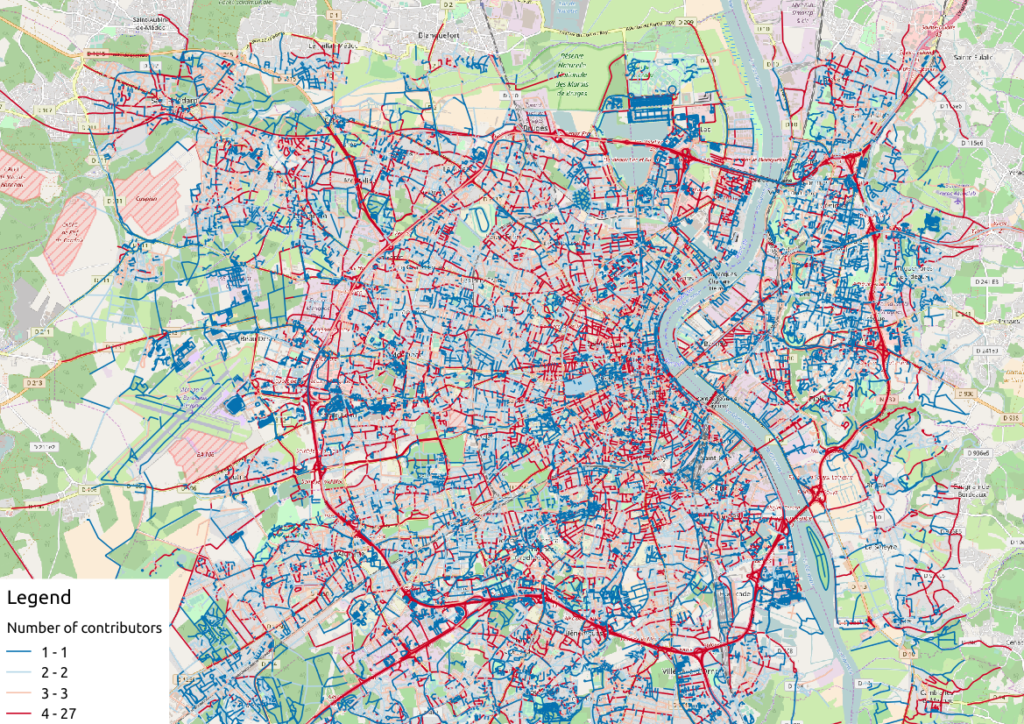
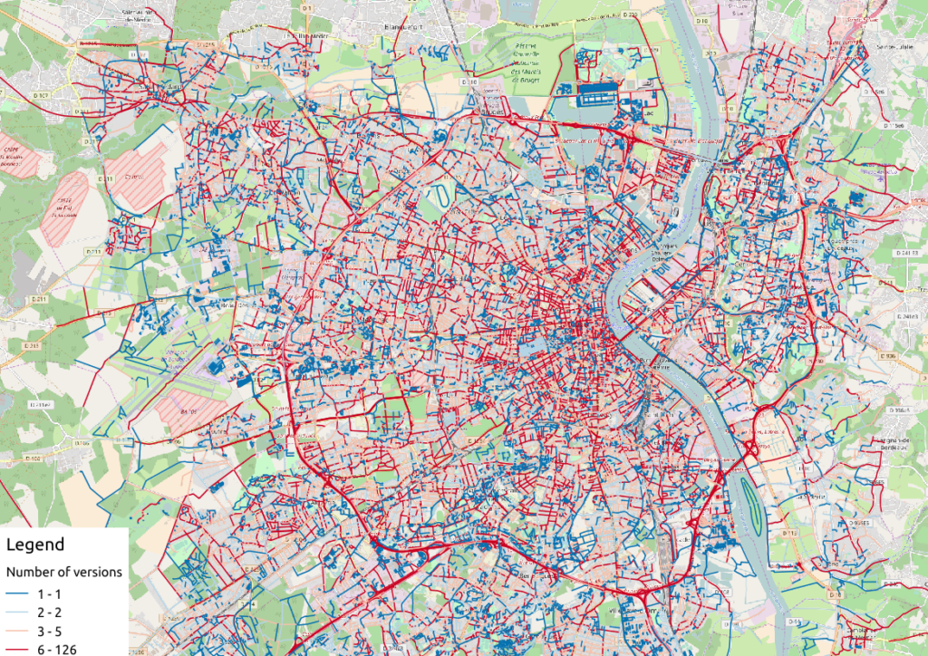
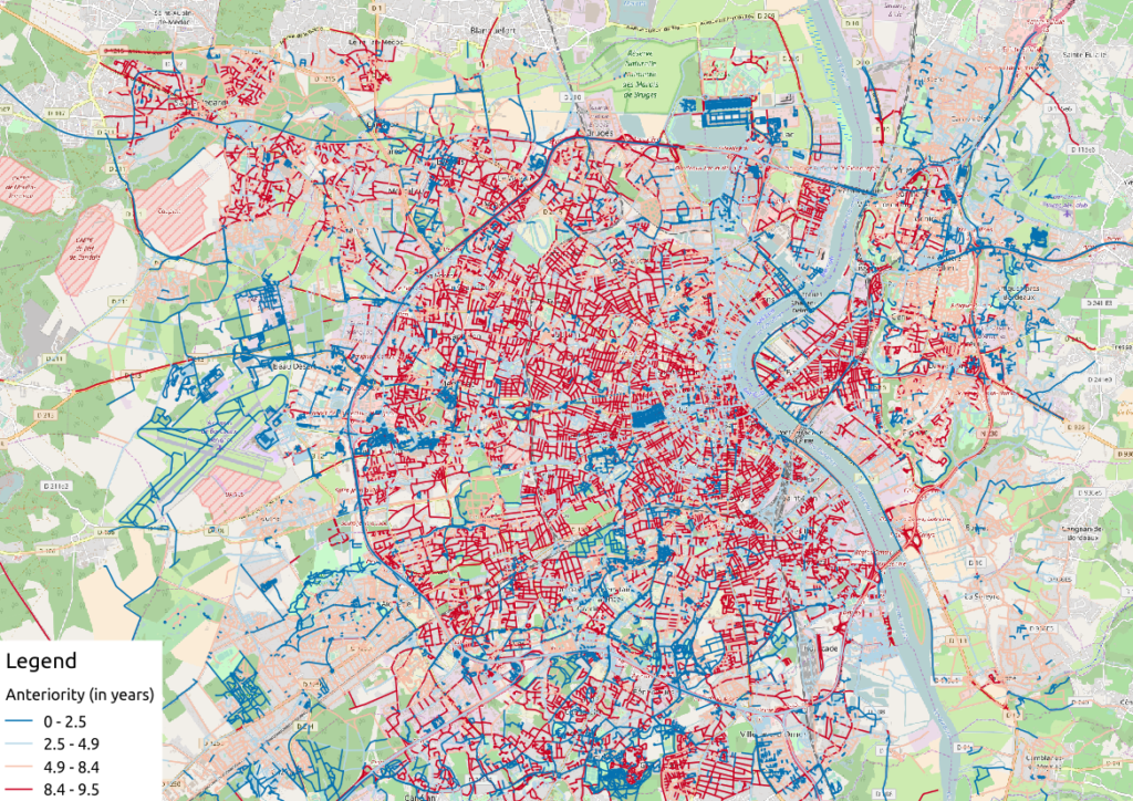
As a first insight on OSM elements, we can plot each OSM ways regarding simple features like the number of users who have contributed, the number of version or the element anteriority.

Figure 1: Number of active contributors per OSM way in Bordeaux


Figure 2: Number of versions per OSM way in Bordeaux

With the first two maps, we see that the ring around Bordeaux is the most intensively modified part of the road network: more unique contributors are implied in the way completion, and more versions are designed for each element. Some major roads within the city center present the same characteristics.

Figure 3: Anteriority of each OSM way in Bordeaux, in years

If we consider the anteriority of OSM roads, we have a different but interesting insight of the area. The oldest roads are mainly located within the city center, even if there are some exceptions. It is also interesting to notice that some spatial patterns arise with temporality: entire neighborhoods are mapped within the same anteriority.

2.2 More complex: OSM data merging with alternative geospatial representations

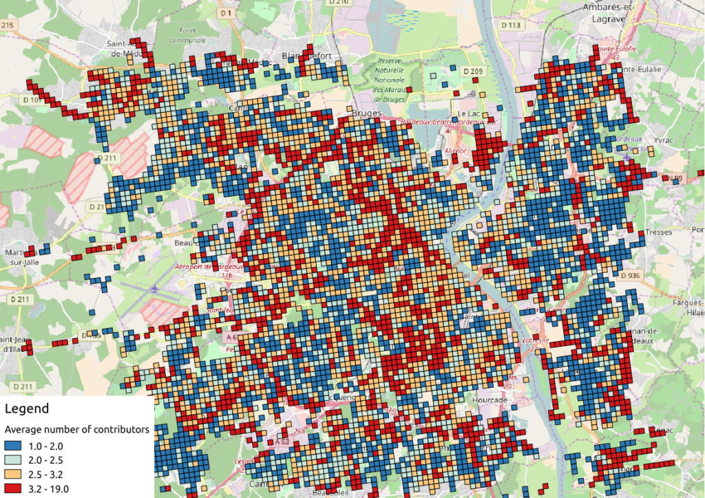
To go deeper into the mapping analysis, we can use the INSEE carroyed data, that divides France into 200-meter squared tiles. As a corollary OSM element statistics may be aggregated into each tile, to produce additional maps. Unfortunately an information loss will occur, as such tiles are only defined where people lives. However it can provides an interesting alternative illustration.

To exploit such new data set, we have to merge the previous table with the accurate INSEE table. Creating indexes on them is of great interest before running such a merging operation:

CREATE INDEX insee_geom_gist
ON open_data.insee_200_carreau USING GIST(wkb_geometry);
CREATE INDEX osm_geom_gist
ON bordeaux_metropole_geomelements USING GIST(geom);

DROP TABLE IF EXISTS bordeaux_metropole_carroyed_ways;
CREATE TABLE bordeaux_metropole_carroyed_ways AS (
SELECT insee.ogc_fid, count(*) AS nb_ways,
avg(bm.version) AS avg_version, avg(bm.lifespan) AS avg_lifespan,
avg(bm.n_days_since_creation) AS avg_anteriority,
avg(bm.n_users) AS avg_n_users, avg(bm.n_chgsets) AS avg_n_chgsets,
insee.wkb_geometry AS geom
FROM open_data.insee_200_carreau AS insee
JOIN bordeaux_metropole_geomelements AS bm
ON ST_Intersects(insee.wkb_geometry, bm.geom)
GROUP BY insee.ogc_fid
);

As a consequence, we get only 5468 individuals (tiles), a quantity that must be compared to the 29427 roads previously handled… This operation will also simplify the map analysis!

We can propose another version of previous maps by using Qgis, let’s consider the average number of contributors per OSM roads, for each tile:

Figure 4: Number of contributors per OSM roads, aggregated by INSEE tile

2.3 The cherry on the cake: representation of OSM elements with respect to quality

Last but not least, the information about last user cluster can shed some light on OSM data quality: by plotting each roads according to the last user who has contributed, we might identify questionable OSM elements!

We simply have to design similar map than in previous section, with user classification information:

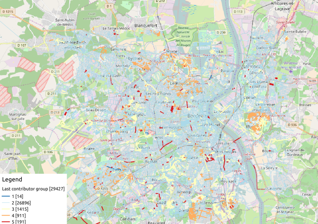
Figure 5: OSM roads around Bordeaux, according to the last user cluster (1: C1, relation experts; 2: C0, versatile expert contributors; 3: C4, recent one-shot way contributors; 4: C3, old one-shot way contributors; 5: C5, locally-unexperienced way specialists)

According to the clustering done in the previous article (be careful, the legend is not the same here…), we can make some additional hypothesis:

  • Light-blue roads are OK, they correspond to the most trustful cluster of contributors (91.4% of roads in this example)
  • There is no group-0 road (group 0 corresponds to cluster C2 in the previous article)… And that’s comforting! It seems that “untrustworthy” users do not contribute to roads or -more probably- that their contributions are quickly amended.
  • Other contributions are made by intermediate users: a finer analysis should be undertaken to decide if the corresponding elements are valid. For now, we can consider everything is OK, even if local patterns seem strong. Areas of interest should be verified (they are not necessarily of low quality!)

For sure, it gives a fairly new picture of OSM data quality!

3 Conclusion

In this last article, we have designed new maps on a small area, starting from element metadata. You have seen the conclusion of our analysis: characterizing the OSM data quality starting from the user contribution history.

Of course some works still have to be done, however we detailed a whole methodology to tackle the problem. We hope you will be able to reproduce it, and to design your own maps!

Feel free to contact us if you are interested in this topic!

The EuroLST seamless and gap-free daily European maps of land surface temperatures

The EuroLST dataset is seamless and gap-free with a temporal resolution of four records per day and enhanced spatial resolution of 250 m. This newly developed reconstruction method (Metz et al, 2014) has been applied to Europe and neighbouring countries, resulting in complete daily coverage from 2001 onwards. To our knowledge, this new reconstructed LST time series exceeds the level of detail of comparable reconstructed LST datasets by several orders of magnitude. Studies on emerging diseases, parasite risk assessment and temperature anomalies can now be performed on the continental scale, maintaining high spatial and temporal detail. In their paper, the authors provide examples for implications and applications of the new LST dataset, such as disease risk assessment, epidemiology, environmental monitoring, and temperature anomalies.

Reconstructed MODIS Land Surface Temperature Dataset, at 250m pixel resolution (click figure to enlarge):
MODIS lst time series reconstructed

Section 1. Article and data citation:

EuroLST has been produced by the former PGIS group at Fondazione Edmund Mach, DBEM based on daily MODIS LST (Product of NASA) maps.

Metz, M.; Rocchini, D.; Neteler, M. 2014: Surface temperatures at the continental scale: Tracking changes with remote sensing at unprecedented detail. Remote Sensing. 2014, 6(5): 3822-3840 (DOI | HTML | PDF)

Section 2. Used software

Open Source commands used in processing (GRASS GIS 7):
links to the related manual pages involved in the data preparation

  • i.pca: Principal Components Analysis (PCA) for image processing.
  • r.regression.multi: it calculates multiple linear regression from raster maps
  • v.surf.bspline: it performs bicubic or bilinear spline interpolation with Tykhonov regularization.

Furthermore:

  • r.bioclim: calculates various bioclimatic indices from monthly temperature and optional precipitation time series (install in GRASS GIS 7 with “g.extention r.bioclim”)
  • pyModis: Free and Open Source Python based library to work with MODIS data

Section 3. Metadata

Map projection: EPSG 3035, prj file
PROJCS["Lambert Azimuthal Equal Area",
    GEOGCS["grs80",
        DATUM["European_Terrestrial_Reference_System_1989",
            SPHEROID["Geodetic_Reference_System_1980",6378137,298.257222101]],
        PRIMEM["Greenwich",0],
        UNIT["degree",0.0174532925199433]],
    PROJECTION["Lambert_Azimuthal_Equal_Area"],
    PARAMETER["latitude_of_center",52],
    PARAMETER["longitude_of_center",10],
    PARAMETER["false_easting",4321000],
    PARAMETER["false_northing",3210000],
    UNIT["Meter",1]]

1. Selected open data derived from EuroLST

Section 1. BIOCLIM derived from reconstructed MODIS LST at 250m pixel resolution

BIO1: Annual mean temperature (°C*10) BIO2: Mean diurnal range (Mean monthly (max - min tem)) BIO3: Isothermality ((bio2/bio7)*100) BIO4: Temperature seasonality (standard deviation * 100) BIO5: Maximum temperature of the warmest month (°C*10) BIO6: Minimum temperature of the coldest month (°C*10) BIO7: Temperature annual range (bio5 - bio6) (°C*10) BIO10: Mean temperature of the warmest quarter (°C*10) BIO11: Mean temperature of the coldest quarter (°C*10)

BIOCLIM-like European LST maps following the “Bioclim” definition (Hutchinson et al., 2009) – derived from 10 years of reconstructed MODIS LST (download to be completed) as GeoTIFF files, 250m pixel resolution, in EU LAEA projection:

Each ZIP file contains the respective GeoTIFF file (for cell value units, see below), the color table as separate ASCII file and a README.txt with details.

Section 2. WMS/WCS Server

Using this URL, you can read the EuroLST BIOCLIM data directly via OGC WMS and WCS protocol:

http://geodati.fmach.it/production/ows_europe_lst

Section 3. OpenData License

The data published in this page are open data and released under the ODbL (Open Database License).

The full EuroLST dataset is not released online as open data (size: 18TB), please ask Luca Delucchi or Roberto Zorer for more info


2. Acknowledgments

The MOD11A1.005, MYD11A1.005 were retrieved from the online web site, courtesy of the NASA EOSDIS Land Processes Distributed Active Archive Center (LP DAAC), USGS/Earth Resources Observation and Science (EROS) Center, Sioux Falls, South Dakota, http://e4ftl01.cr.usgs.gov/

The post The EuroLST seamless and gap-free daily European maps of land surface temperatures appeared first on GFOSS Blog | GRASS GIS Courses.

Using the 25m EU-DEM for shading OpenStreetMap layers

Inspired by Václav Petráš posting about “Did you know that you can see streets of downtown Raleigh in elevation data from NC sample dataset?” I wanted to try the new GRASS GIS 7 Addon r.shaded.pca which creates shades from various directions and combines then into RGB composites just to see what happens when using the new EU-DEM at 25m.

To warm up, I registered the “normally” shaded DEM (previously generated with gdaldem) with r.external in a GRASS GIS 7 location (EPSG 3035, LAEA) and overlayed the OpenStreetMap layer using WMS with GRASS 7′s r.in.wms. An easy task thanks to University of Heidelberg’s www.osm-wms.de. Indeed, they offer a similar shading via WMS, however, in the screenshot below you see the new EU data being used for controlling the light on our own:

OpenStreetMap shaded with EU DEM 25m

OpenStreetMap shaded with EU DEM 25m (click to enlarge)

Next item: trying r.shaded.pca… It supports multi-core calculation and the possibility to strengthen the effects through z-rescaling. In my example, I used:

r.shaded.pca input=eu_dem_25 output=eu_dem_25_shaded_pca nproc=3 zmult=50

The leads to a colorized hillshading map, again with the OSM data on top (50% transparency):

eu_dem_25m_PCA_shaded_OSM_trento_rovereto_garda_lake

OpenStreetMap shaded with r.shaded.pca using EU DEM 25m (click to enlarge)

Yes, fun – I like it :-)

Data sources:

The post Using the 25m EU-DEM for shading OpenStreetMap layers appeared first on GFOSS Blog | GRASS GIS Courses.

EU-DEM: new Digital Surface Model at 25m

eu_dem_upper_garda_lake_riva_arco_italy

EU DEM 25m upper Garda Lake area with Riva del Garda and Arco (Italy). 3D view in wxNVIZ – GRASS GIS 7

The 25m European Digital Elevation Model (EU-DEM, Version 1) is a Digital Surface Model (DSM) representing the first surface as illuminated by the sensors:

eu_dem_s_michele_rotaliana_italy

EU DEM Rotaliana with Mezzocorona and S. Michele (Italy). Produced using Copernicus data and information funded by the European Union – EU-DEM layers.

Its elevations were captured at 1 arc second postings (2.78E-4 degrees). The tiles are provided at 25m resolution in EU-LAEA (EPSG. 3035) projection, temporal coverage: 2000, published in Oct 2013. It is a realisation of the Copernicus programme, managed by the European Commission, DG Enterprise and Industry. Metadata are provided here. According to their “Methodology” page it is a hybrid product based on SRTM and ASTER GDEM data fused by a weighted averaging approach and it has been generated as a contiguous dataset divided into 1 degree by 1 degree tiles, corresponding to the SRTM naming convention. In addition to the DEM data, a colour shaded relief image over Europe is provided.

From the metadata page: “The EU-DEM data are provided as is, i.e. without a formal validation yet. An independent statistical validation is scheduled as part of the GIO land monitoring service activities, and will be made available in the course of 2014.

1. Data download

Note that the GeoTIFF files are of major size, up to 5 GB:

Hint for GRASS GIS users: instead of importing the data, you can use r.external to simply register the GeoTIFF file within a EU LAEA projected location.

eu_dem_trento_adige_s_michele_italy

The post EU-DEM: new Digital Surface Model at 25m appeared first on GFOSS Blog | GRASS GIS Courses.

Processing Landsat 8 data in GRASS GIS 7: Import and visualization

banner_landsat_rgb

For our analysis example, we’ll obtain (freely – thanks, NASA and USGS!) a Landsat 8 scene from http://earthexplorer.usgs.gov/

First of all, you should register.

1. Landsat 8 download procedure

1. Enter Search Criteria:

  • path/row tab, enter Type WRS2: Path: 16, Row: 35
  • Date range: 01/01/2013 – today
  • Click on the “Data sets >>” button

2. Select Your Data Set(s):

  • Expand the entry + Landsat Archive
        [x] L8 OLI/TIRS
  • Click on the “Results >>” button

(We jump over the additional criteria)

4. Search Results

From the resulting list, we pick the data set:

earthexplorer_selection_lsat8Entity ID: LC80160352013134LGN03
Coordinates: 36.04321,-79.28696
Acquisition Date: 14-MAY-13

Using the “Download options”, you can download the data set (requires login). Select the choice:
[x] Level 1 GeoTIFF Data Product (842.4 MB)

You will receive the file “LC80160352013134LGN03.tar.gz”.

2. Unpacking the downloaded Landsat 8 dataset

To unpack the data, run (or use a graphical tool at your choice):

tar xvfz LC80160352013134LGN03.tar.gz

A series of GeoTIFF files will be extracted: LC80160352013134LGN03_B1.TIF, LC80160352013134LGN03_B2.TIF, LC80160352013134LGN03_B3.TIF, LC80160352013134LGN03_B4.TIF, LC80160352013134LGN03_B5.TIF, LC80160352013134LGN03_B6.TIF, LC80160352013134LGN03_B7.TIF, LC80160352013134LGN03_B8.TIF, LC80160352013134LGN03_B9.TIF, LC80160352013134LGN03_B10.TIF, LC80160352013134LGN03_B11.TIF, LC80160352013134LGN03_BQA.TIF

We may check the metadata with “gdalinfo“:

gdalinfo LC80160352013134LGN03_B1.TIF
Driver: GTiff/GeoTIFF
Files: LC80160352013134LGN03_B1.TIF
Size is 7531, 7331
Coordinate System is:
PROJCS["WGS 84 / UTM zone 17N",
    GEOGCS["WGS 84",
        DATUM["WGS_1984",
            SPHEROID["WGS 84",6378137,298.257223563,
...
Pixel Size = (30.000000000000000,-30.000000000000000)
...

3. Want to spatially subset the Landsat scene first?

If you prefer to cut out a smaller area (subregion), check here for gdal_translate usage examples.

4. Import into GRASS GIS 7

Note: While this Landsat 8 scene covers the area of the North Carolina (NC) sample dataset, it is delivered in UTM rather than the NC's state plane metric projection. Hence we preprocess the data first in its original UTM projection prior to the reprojection to NC SPM.

Using the Location Wizard, we can import the dataset easily into a new location (in case you don't have UTM17N not already created earlier):

grass70 -gui

grass7_loc_wizard1
grass7_loc_wizard2
grass7_loc_wizard3
grass7_loc_wizard4
grass7_loc_wizard5
grass7_loc_wizard6
grass7_loc_wizard7
grass7_loc_wizard8
grass7_loc_wizard9


Now start GRASS GIS 7 and you will find the first band already imported (the others will follow shortly!).

For the lazy folks among us, we can also create a new GRASS GIS Location right away from the dataset on command line:

grass70 -c LC80160352013134LGN03_B10.TIF ~/grassdata/utm17n

5. Importing the remaining Landsat 8 bands

The remaining bands can be easily imported with the raster import tool:

grass7_import1

The bands can now be selected easily for import:

grass7_import2

  • Select "Directory" and navigate to the right one
  • The available GeoTIFF files will be shown automatically
  • Select those you want to import
  • You may rename (double-click) the target name for each band
  • Extend the computation region accordingly automatically

Click on "Import" to get the data into the GRASS GIS location. This takes a few minutes. Close the dialog window then.

In the "Map layers" tab you can select the bands to be shown:

grass7_visualize1

6. The bands of Landsat 8

(cited from USGS)

Landsat 8 Operational Land Imager (OLI) and Thermal Infrared Sensor (TIRS) images consist of nine spectral bands with a spatial resolution of 30 meters for Bands 1 to 7 and 9. New band 1 (ultra-blue) is useful for coastal and aerosol studies. New band 9 is useful for cirrus cloud detection. The resolution for Band 8 (panchromatic) is 15 meters. Thermal bands 10 and 11 are useful in providing more accurate surface temperatures and are collected at 100 meters. Approximate scene size is 170 km north-south by 183 km east-west (106 mi by 114 mi).

Landsat 8 Operational Land Imager (OLI) and Thermal Infrared Sensor (TIRS)Launched February 11, 2013 Bands Wavelength (micrometers) Resolution (meters)
Band 1 - Coastal aerosol 0.43 - 0.45 30
Band 2 - Blue 0.45 - 0.51 30
Band 3 - Green 0.53 - 0.59 30
Band 4 - Red 0.64 - 0.67 30
Band 5 - Near Infrared (NIR) 0.85 - 0.88 30
Band 6 - SWIR 1 1.57 - 1.65 30
Band 7 - SWIR 2 2.11 - 2.29 30
Band 8 - Panchromatic 0.50 - 0.68 15
Band 9 - Cirrus 1.36 - 1.38 30
Band 10 - Thermal Infrared (TIRS) 1 10.60 - 11.19 100
Band 11 - Thermal Infrared (TIRS) 2 11.50 - 12.51 100

* TIRS bands are acquired at 100 meter resolution, but are resampled to 30 meter in delivered data product.

7. Natural color view (RGB composite)

Due to the introduction of a new "Cirrus" band (#1), the BGR bands are now 2, 3, and 4, respectively. See also "Common band combinations in RGB" for Landsat 7 or Landsat 5, and Landsat 8.

From Digital Numer (DN) to reflectance:
Before creating an RGB composite, it is important to convert the digital number data (DN) to reflectance (or optionally radiance). Otherwise the colors of a "natural" RGB composite do not look convincing but rather hazy (see background in the next screenshot). This conversion is easily done using the metadata file which is included in the data set with i.landsat.toar:

grass7_landsat_toar0
grass7_landsat_toar1
grass7_landsat_toar2
grass7_landsat_toar3

Now we are ready to create a nice RGB composite:

grass7_landsat_rgb0

grass7_landsat_rgb1

Select the bands to be visually combined:

grass7_visualize2

... and voilà!

grass7_landsat_rgb2

8. Applying the Landsat 8 Quality Assessment (QA) Band

One of the bands of a Landsat 8 scene is named "BQA" which contains for each pixel a decimal value representing a bit-packed combination of surface, atmosphere, and sensor conditions found during the overpass.  It can be used to judge the overall usefulness of a given pixel.

We can use this information to easily eliminate e.g. cloud contaminated pixels. In short, the QA concept is (cited here from the USGS page):

Cited from http://landsat.usgs.gov/L8QualityAssessmentBand.php‎

For the single bits (0, 1, 2, and 3):
0 = No, this condition does not exist
1 = Yes, this condition exists.

The double bits (4-5, 6-7, 8-9, 10-11, 12-13, and 14-15) represent levels of confidence that a condition exists:
00 = Algorithm did not determine the status of this condition
01 = Algorithm has low confidence that this condition exists (0-33 percent confidence)
10 = Algorithm has medium confidence that this condition exists (34-66 percent confidence)
11 = Algorithm has high confidence that this condition exists (67-100 percent confidence).

Detailed bit patterns (d: double bits; s: single bits):
d  Bit 15 = 0 = cloudy
d  Bit 14 = 0 = cloudy
d  Bit 13 = 0 = not a cirrus cloud
d  Bit 12 = 0 = not a cirrus cloud
d  Bit 11 = 0 = not snow/ice
d  Bit 10 = 0 = not snow/ice
d  Bit 9 = 0 = not populated
d  Bit 8 = 0 = not populated
d  Bit 7 = 0 = not populated
d  Bit 6 = 0 = not populated
d  Bit 5 = 0 = not water
d  Bit 4 = 0 = not water
s  Bit 3 = 0 = not populated
s  Bit 2 = 0 = not terrain occluded
s  Bit 1 = 0 = not a dropped frame
s  Bit 0 = 0 = not fill

Usage example 1:  Creating a mask from a bitpattern

We can create a cloud mask (bit 15+14 are set) from this pattern:
cloud:   1100000000000000

Using the Python shell tab, we can easily convert this into the corresponding decimal number for r.mapcalc:

Cited from http://landsat.usgs.gov/L8QualityAssessmentBand.php‎

Welcome to wxGUI Interactive Python Shell 0.9.8

Type "help(grass)" for more GRASS scripting related information.
Type "AddLayer()" to add raster or vector to the layer tree.

Python 2.7.5 (default, Aug 22 2013, 09:31:58) 
[GCC 4.8.1 20130603 (Red Hat 4.8.1-1)] on linux2
Type "help", "copyright", "credits" or "license" for more information.
>>> int(0b1100000000000000)
49152

Using this decimal value of 49152, we can create a cloud mask:

# set NULL for cloudy pixels, 1 elsewhere:
r.mapcalc "cloudmask = if(LC80160352013134LGN03_BQA == 49152, null(), 1 )"

# apply this mask
r.mask cloudmask

In our sample scene, there are only tiny clouds in the north-east, so no much to be seen. Some spurious cloud pixels are scattered over the scene, too, which could be eliminated (in case of false positives) or kept.

Usage example 2:  Querying the Landsat 8 BQA map and retrieve the bitpattern

Perhaps you prefer to query the BQA map itself (overlay the previously created RGB composite and query the BSA map by selecting it in the Layer Manager). In our example, we query the BQA value of the cloud:

Using again the Python shell tab, we can easily convert the decimal number (used for r.mapcalc) into the corresponding binary representation to verify with the  table values above.

>>> x=61440
>>> print(bin(x & 0xffffffff))
0b1111000000000000

Hence, bits 15,14,13, and 12 are set: cloudy and not a cirrus cloud. Looking at the RGB composite we tend to agree :-) Time to mask out the cloud!

wxGUI menu >> Raster >> Mask [r.mask]

Or use the command line, as shown already above:

# remove existing mask (if active)
r.mask -r

# set NULL for cloudy pixels, 1 elsewhere:
r.mapcalc "cloudmask = if(LC80160352013134LGN03_BQA == 61440, null(), 1 )" --o

# apply the new mask
r.mask cloudmask

The visual effect in the RGB composite is minimal since the cloud is white anyway (as NULL cells, too). However, it is relevant for real calculations such as NDVI (vegetation index) or thermal maps.

We observe dark pixels around the cloud originating from thin clouds. In a subsequent identification/mask step we may eliminate also those pixels with a subsequent filter.
  • Page 1 of 1 ( 6 posts )
  • data

Back to Top

Sustaining Members