During the pandemic, people noticed how well they could work remotely, how productive meetings via video call could be, and how well webinars worked. At OPENGIS.ch, this wasn’t news because we have always been 100% remote. However, we missed the unplanned, in-person interactions that occur during meetups with a or . That’s why we’re very pleased that last week we could join the Swiss QGIS user day for the second time after the pandemic.

OPENGIS.ch has been invested in QGIS since its inception in 2014, actually even before; our CEO Marco started working with QGIS 0.6 in 2004 and our CTO Matthias with version 1.7 in 2012. Since 2019, we have also been the company with the most core committers. We can definitely say that OPENGIS.ch has been one of the main driving forces behind the large adoption of QGIS in Switzerland and worldwide. 

Looking at the work done in the QGIS code we’re by far the most prolific company in Switzerland and second worldwide only to North Road Consulting. On top of it, we were the first – and still only one of two- companies to sustain QGIS.org at a Large level since 2021.

This makes us very proud and it is why we’re even happier to see how much that is happening around QGIS in Switzerland aligns with the visions and goals we set out to reach years ago.

The morning started with a presentation by our CTO Matthias “What’s new in QGIS” featuring plenty of work sponsored by the Anwendergruppe CH.

DXF Improvements, the release of SwissLocator 3.0 with swissalti3d and vector tiles integration, and an update on the advances towards solid curve handling in QGIS, a prerequisite for properly handling AV data in Switzerland, were only some of the many noteworthy points he touched.

The highlight of Matthias’ presentation was the better OGC API Features support in QGIS, which was also highlighted in a subsequent talk about Kablo, showing how the next generation of industry solutions (Fachschalen) will be implemented.

Slides: Neues aus der QGIS Welt - QGIS Anwendertag 2024

Following was a short presentation on the project DMAV, Christoph Lauber introduced a project that aims to implement an industry solution for official cadastral surveying with QGIS.

Adrian Wicki of the Federal Office for the Environment (FOEN) and Isabel presented how OPENGIS.ch and the partners Puzzle and Zeilenwerk help the FOEN with the SAM project with assess the hazards of flood, forest fire, or landslides, and warn authorities and the population. With an agile project organisation, the complex project succeeds in fulfilling requirements by applying user-centred development concepts. QGIS is used for visualizing and analyzing data and helping forecasters gain insights into the current situation.

Slides: BAFU_SAM

Andreas Neumann from ETH Zurich and Michael presented the qgis-js project. QGIS-js is an effort to port QGIS core to WebAssembly so that it can be run in a web browser. Although still in the early experimentation phase, this project has great potential to leverage interesting new use cases that weren’t even thinkable before.

Slides: https://boardend.github.io/qgis-js-demo/ 

Olivier Monod from the City of Yverdon presented Kablo, an electricity management proof of concept of the next generation implementation for industry solutions developed in collaboration with OPENGIS.ch.

By applying a middleware based on OGC API Features and Django, Kablo shows how common limitations of current industry solutions (like permission management and atomic operations) can be overcome and how the future brings desktop and web closer together.

Slides: kablo-qgis-user-days

Obviously, it wasn’t just OPENGIS.ch. Sandro Mani from Sourcepole presented the latest and greatest improvements on QWC2, like street view integration and cool QGIS features brought to a beautiful web gis. Andreas Schmid from Kt. Solothurn presented how cool cloud-optimized geotiff (COG) is and what challenges come with it. Interested in the topic? Read more in our report about cloud optimized formats. Mattia Panduri from Canton Ticino explained how they used QGIS to harmonise the cantonal building datasets and Timothée Produit from IG Group SA presented how pic2map helps bring photos to maps. 

To round up the morning, Nyall Dawson from North Road Consulting did a live session around the world to show the latest developments around elevation filtering in QGIS.

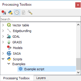
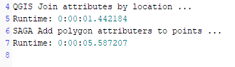
In the afternoon, workshops followed. Claas Leiner led a QGIS expression one while Matthias and Michael showed how to leverage QGIS processing for building geospatial data processing workflows. 

The first QGIS model baker user meeting took place in the third room. The participants discussed this fantastic tool we developed to make INTERLIS work smarter and more productive.

It was a very rich and constructive QGIS user day. We came home with plenty of new ideas and a sense of fulfilment, seeing how great the community we observed and helped grow has become.

A big thanks go to the organisers and everyone involved in making such a great event happen. Only the beer in the sunshine was literally watered by the rain. Nevertheless, there were exciting discussions in the station bistro or in the restaurant coaches on the way home.

See you next time and keep contributing

Today’s post is a geeky deep dive into how to leverage DVC (not just) data version control to track QGIS geoprocessing workflows.

“Why is this great?” you may ask.

DVC tracks data, parameters, and code. If anything changes, we simply rerun the process and DVC will figure out which stages need to be recomputed and which can be skipped by re-using cached results.

This can lead to huge time savings compared to re-running the whole model

You can find the source code used in this post on my repo https://github.com/anitagraser/QGIS-resources/tree/dvc

I’m using DVC with the DVC plugin for VSCode but DVC can be used completely from the command line, if you prefer this appraoch.

Basically, what follows is a proof of concept: converting a QGIS Processing model to a DVC workflow. In the following screenshot, you can see the main stages

1. The QGIS model in the upper left corner
2. The Python script exported from the QGIS model builder in the lower left corner
3. The DVC stages in my dvc.yaml file in the upper right corner (And please ignore the hello world stage. It’s a left over from my first experiment)
4. The DVC DAG visualizing the sequence of stages. Looks similar to the QGIS model, doesn’t it ;-)

Besides the stage definitions in dvc.yaml, there’s a parameters file:

random-points:
  n: 10
buffer-points:
  size: 0.5

And, of course, the two stages, each as it’s own Python script.

First, random-points.py which reads the random-points.n parameter to create the desired number of points within the polygon defined in qgis3/data/test.geojson:

import dvc.api

from qgis.core import QgsVectorLayer
from processing.core.Processing import Processing
import processing

Processing.initialize()

params = dvc.api.params_show()
pts_n = params['random-points']['n']

input_vector = QgsVectorLayer("qgis3/data/test.geojson")
output_filename = "qgis3/output/random-points.geojson"

alg_params = {
    'INCLUDE_POLYGON_ATTRIBUTES': True,
    'INPUT': input_vector,
    'MAX_TRIES_PER_POINT': 10,
    'MIN_DISTANCE': 0,
    'MIN_DISTANCE_GLOBAL': 0,
    'POINTS_NUMBER': pts_n,
    'SEED': None,
    'OUTPUT': output_filename
}
processing.run('native:randompointsinpolygons', alg_params)

And second, buffer-points.py which reads the buffer-points.size parameter to buffer the previously generated points:

import dvc.api
import geopandas as gpd
import matplotlib.pyplot as plt

from qgis.core import QgsVectorLayer
from processing.core.Processing import Processing
import processing

Processing.initialize()

params = dvc.api.params_show()
buffer_size = params['buffer-points']['size']

input_vector = QgsVectorLayer("qgis3/output/random-points.geojson")
output_filename = "qgis3/output/buffered-points.geojson"

alg_params = {
    'DISSOLVE': False,
    'DISTANCE': buffer_size,
    'END_CAP_STYLE': 0,  # Round
    'INPUT': input_vector,
    'JOIN_STYLE': 0,  # Round
    'MITER_LIMIT': 2,
    'SEGMENTS': 5,
    'OUTPUT': output_filename
}
processing.run('native:buffer', alg_params)

gdf = gpd.read_file(output_filename)
gdf.plot()

plt.savefig('qgis3/output/buffered-points.png')

With these things in place, we can use dvc to run the workflow, either from within VSCode or from the command line. Here, you can see the workflow (and how dvc skips stages and fetches results from cache) in action:

If you try it out yourself, let me know what you think.

Amongst all the processing algorithms already available in QGIS, sometimes the one thing you need is missing. 

This happened not a long time ago, when we were asked to find a way to continuously visualise traffic on the Swiss motorway network (polylines) using frequently measured traffic volumes from discrete measurement stations (points) alongside the motorways. In order to keep working with the existing polylines, and be able to attribute more than one value of traffic to each feature, we chose to work with the M-values. M-values are a per-vertex attribute like X, Y or Z coordinates. They contain a measure value, which typically represents time or distance. But they can hold any numeric value.

In our example, traffic measurement values are provided on a separate point layer and should be attributed to the M-value of the nearest vertex of the motorway polylines. Of course, the motorway features should be of type LineStringM in order to hold an M-value. We then should interpolate the M-values for each feature over all vertices in order to get continuous values along the line (i.e. a value on every vertex). This last part is not yet existing as a processing algorithm in QGIS.

This article describes how to write a feature-based processing algorithm based on the example of M-value interpolation along LineStrings.

Feature-based processing algorithm

The pyqgis class QgsProcessingFeatureBasedAlgorithm is described as follows: “An abstract QgsProcessingAlgorithm base class for processing algorithms which operates “feature-by-feature”.  

Feature based algorithms are algorithms which operate on individual features in isolation. These are algorithms where one feature is output for each input feature, and the output feature result for each input feature is not dependent on any other features present in the source. […]

Using QgsProcessingFeatureBasedAlgorithm as the base class for feature based algorithms allows shortcutting much of the common algorithm code for handling iterating over sources and pushing features to output sinks. It also allows the algorithm execution to be optimised in future (for instance allowing automatic multi-thread processing of the algorithm, or use of the algorithm in “chains”, avoiding the need for temporary outputs in multi-step models).”

In other words, when connecting several processing algorithms one after the other – e.g. with the graphical modeller – these feature-based processing algorithms can easily be used to fill in the missing bits. 

Compared to the standard QgsProcessingAlgorithm the feature-based class implicitly iterates over each feature when executing and avoids writing wordy loops explicitly fetching and applying the algorithm to each feature. 

Just like for the QgsProcessingAlgorithm (a template can be found in the Processing Toolbar > Scripts > Create New Script from Template), there is quite some boilerplate code in the QgsProcessingFeatureBasedAlgorithm. The first part is identical to any QgsProcessingAlgorithm.

After the description of the algorithm (name, group, short help, etc.), the algorithm is initialised with def initAlgorithm, defining input and output. 

In our M-value example:

    def initAlgorithm(self, config=None):
        self.addParameter(
            QgsProcessingParameterFeatureSource(
                self.INPUT,
                self.tr('Input layer'),
                [QgsProcessing.TypeVectorAnyGeometry]
            )
        )
        self.addParameter(
            QgsProcessingParameterFeatureSink(
                self.OUTPUT,
                self.tr('Output layer')
            )
        )

While in a regular processing algorithm now follows def processAlgorithm(self, parameters, context, feedback), in a feature-based algorithm we use def processFeature(self, feature, context, feedback). This implies applying the code in this block to each feature of the input layer. 

Interpolating M-values

This actual processing part can be copied and added almost 1:1 from any other independent python script, there is little specific syntax to make it a processing algorithm. Only the first line below really.

In our M-value example:

    def processFeature(self, feature, context, feedback):
        
        try:
            geom = feature.geometry()
            line = geom.constGet()
            vertex_iterator = QgsVertexIterator(line)
            vertex_m = []

            # Iterate over all vertices of the feature and extract M-value

            while vertex_iterator.hasNext():
                vertex = vertex_iterator.next()
                vertex_m.append(vertex.m())

            # Extract length of segments between vertices

            vertices_indices = range(len(vertex_m))
            length_segments = [sqrt(QgsPointXY(line[i]).sqrDist(QgsPointXY(line[j]))) 
                for i,j in itertools.combinations(vertices_indices, 2) 
                if (j - i) == 1]

            # Get all non-zero M-value indices as an array, where interpolations 
              have to start

            vertex_si = np.nonzero(vertex_m)[0]
            
            m_interpolated = np.copy(vertex_m)

            # Interpolate between all non-zero M-values - take segment lengths between 
              vertices into account

            for i in range(len(vertex_si)-1):
                first_nonzero = vertex_m[vertex_si[i]]
                next_nonzero = vertex_m[vertex_si[i+1]]
                accum_dist = itertools.accumulate(length_segments[vertex_si[i]
                                                                  :vertex_si[i+1]])
                sum_seg = sum(length_segments[vertex_si[i]:vertex_si[i+1]])
                interp_m = [round(((dist/sum_seg)*(next_nonzero-first_nonzero)) + 
                            first_nonzero,0) for dist in accum_dist]
                m_interpolated[vertex_si[i]:vertex_si[i+1]] = interp_m

            # Copy feature geometry and set interpolated M-values, 
              attribute new geometry to feature

            geom_new = QgsLineString(geom.constGet())
            
            for j in range(len(m_interpolated)):
                geom_new.setMAt(j,m_interpolated[j])
                
            attrs = feature.attributes()
            
            feat_new = QgsFeature()
            feat_new.setAttributes(attrs)
            feat_new.setGeometry(geom_new)

        except Exception:
            s = traceback.format_exc()
            feedback.pushInfo(s)
            self.num_bad += 1
            return []
        
        return [feat_new]

In our example, we get the feature’s geometry, iterate over all its vertices (using the QgsVertexIterator) and extract the M-values as an array. This allows us to assign interpolated values where we don’t have M-values available. Such missing values are initially set to a value of 0 (zero).

We also extract the length of the segments between the vertices. By gathering the indices of the non-zero M-values of the array, we can then interpolate between all non-zero M-values, considering the length that separates the zero-value vertex from the first and the next non-zero vertex.

For the iterations over the vertices to extract the length of the segments between them as well as for the actual interpolation between all non-zero M-value vertices we use the library itertools. This library provides different iterator building blocks that come in quite handy for our use case. 

Finally, we create a new geometry by copying the one which is being processed and setting the M-values to the newly interpolated ones.

And that’s all there is really!

Styling the result via M-values

The last step is styling our output layer in QGIS, based on the M-values (our traffic M-values are categorised from 1 [a lot of traffic -> dark red] to 6 [no traffic -> light green]). This can be achieved by using a Single Symbol symbology with a Marker Line type “on every vertex”. As a marker type, we use a simple round point. Stroke style is “no pen” and Stroke fill is based on an expression:

with_variable(

'm_value', m(point_n($geometry, @geometry_point_num)),

	CASE WHEN @m_value = 6
		THEN color_rgb(140, 255, 159)

		WHEN @m_value = 5
			THEN color_rgb(244, 252, 0)

		WHEN @m_value = 4
			THEN color_rgb(252, 176, 0)

		WHEN @m_value = 3
			THEN color_rgb(252, 134, 0)

		WHEN @m_value = 2
			THEN color_rgb(252, 29, 0)

		WHEN @m_value = 1
			THEN color_rgb(140, 255, 159)

		ELSE
			color_hsla(0,100,100,0)

	END
)

And voilà! Wherever we have enough measurements on one line feature, we get our motorway network continuously coloured according to the measured traffic volume.

One disclaimer at the end: We get this seemingly continuous styling only because of the combination of our “complex” polylines (containing many vertices) and the zoomed-out view of the motorway network. Because really, we’re styling many points and not directly the line itself. But in our case, this is working very well.

If you’d like to make your custom processing algorithm available through the processing toolbox in your QGIS, just put your script in the folder containing the files related to your user profile:

profiles > default > processing > scripts 

You can directly access this folder by clicking on Settings > User Profiles > Open Active Profile Folder in the QGIS menu.

That way, it’s also available for integration in the graphical modeller.

You can download the above-mentioned processing scripts (with numpy and without numpy) here.

Happy processing!

What are we looking for?

We would like to use WMS offline on QField. For that, we need to figure out what is the best way to get a raster from a WMS and which format is the most efficient (size and performance).

In this post we’ll show you is how to generate the ideal raster file from a WMS and the results of our efficiency tests for the the different raster formats.

WMS to GPKG

The simple way

If there is no limitation on the WMS or you need only a small region, here is the easiest process.

1. Request the WMS and store a description file in XML:

gdal_translate "WMS:url" file.xml -of WMS

2. Create a Geopackage from the information in the description file.

gdal_translate -of GPKG file.xml file.gpkg -co TILE_FORMAT=JPEG

That was quite simple, right?

The larger datasets way

If the command takes too much time, it means that it is trying to download too much data and could be caused by downloading higher resolution data than required.
The command might even completely fail if it contains a request for bigger data blocks thant the server allows.

Here is the process to get larger datasets in a simple way. Let’s use a real example:

1. Use gdal_translate "WMS:https://www.gebco.net/data_and_products/gebco_web_services/web_map_service/mapserv?request=getmap&service=wms&crs=EPSG:4326&format=image/jpeg&layers=gebco_latest&version=1.1.0" test.xml -of WMS
2. Open the test.xml file for editing, here you’ll find the parameters of the WMS. We change the “SizeX” to 3600 and “SizeY” to 1800. By changing these parameters we lower the resolution. It is important to keep proportionality.
3. Another thing we need to change are “BlockSizeX” and “BlockSizeY” that define the size of the tiles. We change both to 2048.
4. Finally, use gdal_translate -of GPKG test.xml test.gpkg -co TILE_FORMAT=JPEG
5. To make a Geopackage pyramid use gdaladdo GPKG:test.gpkg:gebco_latest. It will replace the Geopackage, if you want to keep the original one, you need to copy it first.

Now you have a raster Geopackage that you can use in QField.

Testing raster formats

Preparing the files

As first step we exported our test orthophoto WMS to a plain GeoTIFF using QGIS’ default behaviour.

Rendering test results

We have tested many formats, here is a table with the results of the size and rendering speed in QGIS and QField.
To analyze the speed we used qgis_bench.exe -i 10 -p "C:\test\test.qgs" >> "C:\test\test.log.
Qgis_bench is a tool that renders a QGIS project a number of times to get performance measurements. The parameter -i is to define the iterations and -p is the project used which contains only the generated raster.

Analysis

File size

The Geopackage WEBP (with and without pyramid) has the best result for file size, but it is not yet supported by QField (from 1.6) and is only slightly smaller than the JPEG variant.

Plain GeoTiff, MBTiles, Cloud Optimized GeoTIFF (COG – DEFLATE mode) and Geopackages with PNG generate by far the largest file sizes (up to 20x larger) and are thus not recommended.

Rendering speed

MBTiles are on average double as fast as JPEG Geopackages with pyramids which in turn are more than double as fast as GeoTIFF and 15x faster than COG.
Geopackages without pyramids are 200 to 400 times slower.

Conclusion

Even though MBTiles render faster than the Geopackage pyramid JPEG, they come with an almost 10x bigger storage requirement which makes us say that the best offline raster format supported by QField is Geopackage pyramid JPEG or if you need transparency and slightly smaller files Geopackage pyramid WebP.

If you need transparency before QField 1.6, the best results are achieved with Geopackage pyramid PNG_JPEG.

QGIS Processing offers a rich and expandable set of algorithms which can operate on spatial data, along with a powerful Model Designer which allows users to string together these algorithms to create custom workflows.

Since its introduction in QGIS 2, the Processing framework has seen an intensive amount of development and optimisation efforts. In recent QGIS releases it offers a very user-friendly way of performing complex spatial data processing tasks, all without requiring ANY expensive third-party tools or software licenses!

At North Road we are passionate about the QGIS Processing framework, and have invested considerable effort in this framework over the past 5 years. We’re proud to announce that our latest crowd-funding campaign is focused on further expanding the capabilities and flexibility of Processing and the Processing Model Designer!

Unlike a typical crowdfunding campaign, where a specific funding target and deadline is set, we’re running this campaign a little differently. Instead, this campaign is taking the form of a “à la carte” menu of Processing enhancements. These range from small “paper-cut” style fixes, through to larger architectural improvements, and are each individually priced accordingly. We are asking backers to pick individual enhancements from this “menu of enhancements” and fund that enhancement’s development in full. In order to make this campaign affordable for a wide range of backers, we’ve included a huge range of enhancements which vary in price from smaller amounts to larger amounts.

You can read the full details of the campaign and browse the list of proposed enhancements at the campaign page.

When QGIS 3.0 was release, I published a Processing script template for QGIS3. While the script template is nicely pythonic, it’s also pretty long and daunting for non-programmers. This fact didn’t go unnoticed and Nathan Woodrow in particular started to work on a QGIS enhancement proposal to improve the situation and make writing Processing scripts easier, while – at the same time – keeping in line with common Python styles.

While the previous template had 57 lines of code, the new template only has 26 lines – 50% less code, same functionality! (Actually, this template provides more functionality since it also tracks progress and ensures that the algorithm can be cancelled.)

from qgis.processing import alg
from qgis.core import QgsFeature, QgsFeatureSink

@alg(name="ex_new", label=alg.tr("Example script (new style)"), group="examplescripts", group_label=alg.tr("Example Scripts"))
@alg.input(type=alg.SOURCE, name="INPUT", label="Input layer")
@alg.input(type=alg.SINK, name="OUTPUT", label="Output layer")
def testalg(instance, parameters, context, feedback, inputs):
    """
    Description goes here. (Don't delete this! Removing this comment will cause errors.)
    """
    source = instance.parameterAsSource(parameters, "INPUT", context)

    (sink, dest_id) = instance.parameterAsSink(
        parameters, "OUTPUT", context,
        source.fields(), source.wkbType(), source.sourceCrs())

    total = 100.0 / source.featureCount() if source.featureCount() else 0
    features = source.getFeatures()
    for current, feature in enumerate(features):
        if feedback.isCanceled():
            break
        out_feature = QgsFeature(feature)
        sink.addFeature(out_feature, QgsFeatureSink.FastInsert)
        feedback.setProgress(int(current * total))

    return {"OUTPUT": dest_id}

The key improvement are the new decorators that turn an ordinary function (such as testalg in the template) into a Processing algorithm. Decorators start with @ and are written above a function definition. The @alg decorator declares that the following function is a Processing algorithm, defines its name and assigns it to an algorithm group. The @alg.input decorator creates an input parameter for the algorithm. Similarly, there is a @alg.output decorator for output parameters.

For a longer example script, check out the original QGIS enhancement proposal thread!

For now, this new way of writing Processing scripts is only supported by QGIS 3.6 but there are plans to back-port this improvement to 3.4 once it is more mature. So give it a try and report back!

In Movement data in GIS #16, I presented a new way to deal with trajectory data using GeoPandas and how to load the trajectory GeoDataframes as a QGIS layer. Following up on this initial experiment, I’ve now implemented a first version of an algorithm that performs a spatial analysis on my GeoPandas trajectories.

The first spatial analysis algorithm I’ve implemented is Clip trajectories by extent. Implementing this algorithm revealed a couple of pitfalls:

• To achieve correct results, we need to compute spatial intersections between linear trajectory segments and the extent. Therefore, we need to convert our point GeoDataframe to a line GeoDataframe.
• Based on the spatial intersection, we need to take care of computing the corresponding timestamps of the events when trajectories enter or leave the extent.
• A trajectory can intersect the extent multiple times. Therefore, we cannot simply use the global minimum and maximum timestamp of intersecting segments.
• GeoPandas provides spatial intersection functionality but if the trajectory contains consecutive rows without location change, these will result in zero length lines and those cause an empty intersection result.

So far, the clip result only contains the trajectory id plus a suffix indicating the sequence of the intersection segments for a specific trajectory (because one trajectory can intersect the extent multiple times). The following screenshot shows one highlighted trajectory that intersects the extent three times and the resulting clipped trajectories:

This algorithm together with the basic trajectory from points algorithm is now available in a Processing algorithm provider plugin called Processing Trajectory.

Note: This plugin depends on GeoPandas.

Note for Windows users: GeoPandas is not a standard package that is available in OSGeo4W, so you’ll have to install it manually. (For the necessary steps, see this answer on gis.stackexchange.com)

The implemented tests show how to use the Trajectory class independently of QGIS. So far, I’m only testing the spatial properties though:

def test_two_intersections_with_same_polygon(self):
    polygon = Polygon([(5,-5),(7,-5),(7,12),(5,12),(5,-5)])
    data = [{'id':1, 'geometry':Point(0,0), 't':datetime(2018,1,1,12,0,0)},
        {'id':1, 'geometry':Point(6,0), 't':datetime(2018,1,1,12,10,0)},
        {'id':1, 'geometry':Point(10,0), 't':datetime(2018,1,1,12,15,0)},
        {'id':1, 'geometry':Point(10,10), 't':datetime(2018,1,1,12,30,0)},
        {'id':1, 'geometry':Point(0,10), 't':datetime(2018,1,1,13,0,0)}]
    df = pd.DataFrame(data).set_index('t')
    geo_df = GeoDataFrame(df, crs={'init': '31256'})
    traj = Trajectory(1, geo_df)
    intersections = traj.intersection(polygon)
    result = []
    for x in intersections:
        result.append(x.to_linestring())
    expected_result = [LineString([(5,0),(6,0),(7,0)]), LineString([(7,10),(5,10)])]
    self.assertEqual(result, expected_result) 

One issue with implementing the algorithms as QGIS Processing tools in this way is that the tools are independent of one another. That means that each tool has to repeat the expensive step of creating the trajectory objects in memory. I’m not sure this can be solved.

Remember the good old times when all parameters in Processing were mandatory?

Inputs and outputs are fixed, and optional parameters or outputs are not supported. [Graser & Olaya, 2015]

Since QGIS 2.14, this is no longer the case. Scripts, as well as models, can now have optional parameters. Here is how for QGIS 3:

When defining a Processing script parameter, the parameter’s constructor takes a boolean flag indicating whether the parameter should be optional. It’s false by default:

class qgis.core.QgsProcessingParameterNumber(
   name: str, description: str = '', 
   type: QgsProcessingParameterNumber.Type = QgsProcessingParameterNumber.Integer, 
   defaultValue: Any = None, 
   optional: bool = False,
   minValue: float = -DBL_MAX+1, maxValue: float = DBL_MAX)

(Source: http://python.qgis.org/api/core/Processing/QgsProcessingParameterNumber.html)

One standard tool that uses optional parameters is Add autoincremental field:

From Python, this algorithm can be called with or without the optional parameters:

When building a model, an optional input can be assigned to the optional parameter. To create an optional input, make sure to deactivate the mandatory checkbox at the bottom of the input parameter definition:

Then this optional input can be used in an algorithm. For example, here the numerical input optional_value is passed to the Start values at parameter:

You can get access to all available inputs by clicking the … button next to the Start values at field. In this example, I have access to values of the input layer as well as  the optional value:

Once this is set up, this is how it looks when the model is run:

You can see that the optional value is indeed Not set.

References

Graser, A., & Olaya, V. (2015). Processing: A Python Framework for the Seamless Integration of Geoprocessing Tools in QGIS. ISPRS Int. J. Geo-Inf. 2015, 4, 2219-2245. doi:10.3390/ijgi4042219.

Processing has been overhauled significantly for QGIS 3.0. Besides speed-ups, one of the most obvious changes is the way to write Processing scripts. Instead of the old Processing-specific syntax, Processing scripts for QGIS3 are purely pythonic implementations of QgsProcessingAlgorithm.

Here’s a template that you can use to develop your own algorithms:

from qgis.PyQt.QtCore import QCoreApplication, QVariant
from qgis.core import (QgsField, QgsFeature, QgsFeatureSink, QgsFeatureRequest, QgsProcessing, QgsProcessingAlgorithm, QgsProcessingParameterFeatureSource, QgsProcessingParameterFeatureSink)
                      
class ExAlgo(QgsProcessingAlgorithm):
    INPUT = 'INPUT'
    OUTPUT = 'OUTPUT'

    def __init__(self):
        super().__init__()

    def name(self):
        return "exalgo"
    
    def tr(self, text):
        return QCoreApplication.translate("exalgo", text)
        
    def displayName(self):
        return self.tr("Example script")

    def group(self):
        return self.tr("Examples")

    def groupId(self):
        return "examples"

    def shortHelpString(self):
        return self.tr("Example script without logic")

    def helpUrl(self):
        return "https://qgis.org"
        
    def createInstance(self):
        return type(self)()
  
    def initAlgorithm(self, config=None):
        self.addParameter(QgsProcessingParameterFeatureSource(
            self.INPUT,
            self.tr("Input layer"),
            [QgsProcessing.TypeVectorAnyGeometry]))
        self.addParameter(QgsProcessingParameterFeatureSink(
            self.OUTPUT,
            self.tr("Output layer"),
            QgsProcessing.TypeVectorAnyGeometry))

    def processAlgorithm(self, parameters, context, feedback):
        source = self.parameterAsSource(parameters, self.INPUT, context)
        (sink, dest_id) = self.parameterAsSink(parameters, self.OUTPUT, context,
                                               source.fields(), source.wkbType(), source.sourceCrs())

        features = source.getFeatures(QgsFeatureRequest())
        for feat in features:
            out_feat = QgsFeature()
            out_feat.setGeometry(feat.geometry())
            out_feat.setAttributes(feat.attributes())
            sink.addFeature(out_feat, QgsFeatureSink.FastInsert)

        return {self.OUTPUT: dest_id}

This script just copies the features of the input layer to the output layer without any modifications. Add your logic to the processAlgorithm() function to get started.

Use Create New Script from the Toolbox toolbar:

Paste the example script:

Once saved, the script will show up in the Processing toolbox:

Joining polygon attributes to points based on their location is a very common GIS task. In QGIS 2, QGIS’ own implementation of “Join attributes by location” was much slower than SAGA’s “Add polygon attributes to points”. Thus, installations without SAGA were out of good options.

Luckily this issue (and many more) has been fixed by the rewrite of many geoprocessing algorithms for QGIS 3! Let’s revisit the comparison:

I’m using publicly available datasets from Naturalearth: The small scale populated places (243 points) and the large scale countries (255 polygons with many nodes). Turns out that QGIS 3’s built-in tool takes a little less than two seconds while the SAGA Processing tool requires a litte less than six seconds:

Like in the previous comparison, times were measured using the Python Console:

In both tools, only the countries’ SOVEREIGNT attribute is joined to the point attribute table:

import processing
t0 = datetime.datetime.now()
print("QGIS Join attributes by location ...")
processing.runAndLoadResults(
   "qgis:joinattributesbylocation", 
   {'INPUT':'E:/Geodata/NaturalEarth/vector_v4/natural_earth_vector/110m_cultural/ne_110m_populated_places.shp',
   'JOIN':'E:/Geodata/NaturalEarth/vector_v4/natural_earth_vector/10m_cultural/ne_10m_admin_0_countries.shp',
   'PREDICATE':[5],'JOIN_FIELDS':['SOVEREIGNT'],
   'METHOD':0,'DISCARD_NONMATCHING':False,'OUTPUT':'memory:'})
t1 = datetime.datetime.now()
print("Runtime: "+str(t1-t0))
print("SAGA Add polygon attributers to points ...")
processing.runAndLoadResults("saga:addpolygonattributestopoints", 
   {'INPUT':'E:/Geodata/NaturalEarth/vector_v4/natural_earth_vector/110m_cultural/ne_110m_populated_places.shp',
   'POLYGONS':'E:/Geodata/NaturalEarth/vector_v4/natural_earth_vector/10m_cultural/ne_10m_admin_0_countries.shp',
   'FIELDS':'SOVEREIGNT','OUTPUT':'C:/Users/anita/AppData/Local/Temp/processing_8b1bbde78de5490285dd530e115cca52/099660d88bf14c54a853cc230e388e55/OUTPUT.shp'})
t2 = datetime.datetime.now()
print("Runtime: "+str(t2-t1))

It is worth noting that it takes longer if more attributes are to be joined to the point layer attribute table. For example, if the JOIN_FIELDS parameter is empty:

'JOIN_FIELDS':[]

instead of

'JOIN_FIELDS':['SOVEREIGNT']

then the the Join attributes by location takes almost 16 seconds. (The country layer contains 71 attributes after all.)

(The SAGA tool currently allows only joining one attribute at a time.)

Today’s post is a follow-up of Movement data in GIS #3: visualizing massive trajectory datasets. In that post, I summarized a concept for trajectory generalization. Now, I have published the scripts and sample data in my QGIS-Processing-tools repository on Github.

To add the trajectory generalization scripts to your Processing toolbox, you can use the Add scripts from files tool:

It is worth noting, that Add scripts from files fails to correctly import potential help files for the scripts but that’s not an issue this time around, since I haven’t gotten around to actually write help files yet.

The scripts are used in the following order:

1. Extract characteristic trajectory points
2. Group points in space
3. Compute flows between cells from trajectories

The sample project contains input data, as well as output layers of the individual tools. The only required input is a layer of trajectories, where trajectories have to be LINESTRINGM (note the M!) features:

Trajectory sample based on data provided by the GeoLife project

In Extract characteristic trajectory points, distance parameters are specified in meters, stop duration in seconds, and angles in degrees. The characteristic points contain start and end locations, as well as turns and stop locations:

The characteristic points are then clustered. In this tool, the distance has to be specified in layer units, which are degrees in case of the sample data.

Finally, we can compute flows between cells defined by these clusters:

Flow lines scaled by flow strength and cell centers scaled by counts

If you use these tools on your own data, I’d be happy so see what you come up with!

Read more:

• Movement data in GIS: issues & ideas
• Movement data in GIS #2: visualizing individual trajectories
• Movement data in GIS #3: visualizing massive trajectory datasets
• Movement data in GIS #4: variations over time
• Movement data in GIS #5: current research topics
• Movement data in GIS #6: updates from AGILE2017
• Movement data in GIS #7: animated trajectories with TimeManager
• Movement data in GIS #8: edge bundling for flow maps

Getting a pixel count and area size of unique values for a given raster layer hasn’t been straightforward in QGIS. The user could either go through third-party solutions via processing with some limitations, or create a (slow) python script.

That is, until now. Say hello to the newly-committed processing algorithm, the “raster layer unique values report”.

The QGIS algorithm will take a raster layer as input and output an HTML formatted report listing the pixel count and area size – in the raster layer’s unit - for all unique values. Thanks to QGIS core developer Nyall Dawson’s fantastic work on the processing platform in upcoming QGIS 3.0, the algorithm is written in C++ and therefore much faster - over a tenfold improvement - to an equivalent python script.

Using QGIS’ processing modeler, users can come up with a simple model to provide unique values reports within areas of interests, defined through vector polygons:

For example, using the newly-updated 2016 Global Forest Change dataset and the model above, we can quickly generate a deforestation per year chart. Simply reproject the dataset in the appropriate meter-based projection, clip it with a national boundaries polygon, et voila. Paste the resulting HTML table into your favorite spreadsheet program and enjoy the charts:

It’s been a long time since I last blogged here. Let’s just blame that on the amount of changes going into QGIS 3.0 and move on…

One new feature which landed in QGIS 3.0 today is a processing algorithm for automatic coloring of a map in such a way that adjoining polygons are all assigned different color indexes. Astute readers may be aware that this was possible in earlier versions of QGIS through the use of either the (QGIS 1.x only!) Topocolor plugin, or the Coloring a map plugin (2.x).

What’s interesting about this new processing algorithm is that it introduces several refinements for cartographically optimising the coloring. The earlier plugins both operated by pure “graph” coloring techniques. What this means is that first a graph consisting of each set of adjoining features is generated. Then, based purely on this abstract graph, the coloring algorithms are applied to optimise the solution so that connected graph nodes are assigned different colors, whilst keeping the total number of colors required minimised.

The new QGIS algorithm works in a different way. Whilst the first step is still calculating the graph of adjoining features (now super-fast due to use of spatial indexes and prepared geometry intersection tests!), the colors for the graph are assigned while considering the spatial arrangement of all features. It’s gone from a purely abstract mathematical solution to a context-sensitive cartographic solution.

The “Topological coloring” processing algorithm

Let’s explore the differences. First up, the algorithm has an option for the “minimum distance between features”. It’s often the case that features aren’t really touching, but are instead just very close to each other. Even though they aren’t touching, we still don’t want these features to be assigned the same color. This option allows you to control the minimum distance which two features can be to each other before they can be assigned the same color.

The biggest change comes in the “balancing” techniques available in the new algorithm. By default, the algorithm now tries to assign colors in such a way that the total number of features assigned each color is equalised. This avoids having a color which is only assigned to a couple of features in a large dataset, resulting in an odd looking map coloration.

Balancing color assignment by count – notice how each class has a (almost!) equal count

Another available balancing technique is to balance the color assignment by total area. This technique assigns colors so that the total area of the features assigned to each color is balanced. This mode can be useful to help avoid large features resulting in one of the colors appearing more dominant on a colored map.

Balancing assignment by area – note how only one large feature is assigned the red color

The final technique, and my personal preference, is to balance colors by distance between colors. This mode will assign colors in order to maximize the distance between features of the same color. Maximising the distance helps to create a more uniform distribution of colors across a map, and avoids certain colors clustering in a particular area of the map. It’s my preference as it creates a really nice balanced map – at a glance the colors look “randomly” assigned with no discernible pattern to the arrangement.

Balancing colors by distance

As these examples show, considering the geographic arrangement of features while coloring allows us to optimise the assigned colors for cartographic output.

The other nice thing about having this feature implemented as a processing algorithm is that unlike standalone plugins, processing algorithms can be incorporated as just one step of a larger model (and also reused by other plugins!).

QGIS 3.0 has tons of great new features, speed boosts and stability bumps. This is just a tiny taste of the handy new features which will be available when 3.0 is released!

Hi! In this blog I describe how you can create proper parcels with polygon geometry in from polylines (parcel boundaries) and points (Parcel point with parcel attributes placed inside parcel boundaries). Since the 1st of januari 2016 a dataset named, BRK (Basis Registratie Kadaster) is available from PDOK. You can download these in GML format … Continue reading Generate parcels areas from parcel boundaries

If you follow my blog, you’ve most certainly seen the post How to create illuminated contours, Tanaka-style from earlier this year. As Victor Olaya noted correctly in the comments, the workflow to create this effect lends itself perfectly to being automated with a Processing model.

The model needs only two inputs: the digital elevation model raster and the interval at which we want the contours to be created:

The model steps are straightforward: the contours are generated and split into short segments before the segment orientation is computed using the following code in the Advanced Python Field Calculator:

p1 = $geom.asPolyline()[0]
p2 = $geom.asPolyline()[-1]
a = p1.azimuth(p2)
if a < 0:
   a += 360
value = a

You can find the finished model on Github. Happy QGISing!

In my previous post, I presented a Processing model to determine positional accuracy of street networks. Today, I’ll cover another very popular tool to assess OSM quality in a region: network length comparison. Here’s the corresponding slide from my FOSS4G presentation which shows an example of this approach applied to OSM and OS data in the UK:

One building block of this tool is the Total graph length model which calculates the length of a network within specified regions. Like the model for positional accuracy, this model includes reprojection steps to ensure all layers are in the same CRS before the actual geoprocessing starts:

The final Compare total graph length model combines two instances of “Total graph length” whose results are then joined to eventually calculate the length difference (lenDIFF).

As usual, you can find the models on Github. If you have any questions, don’t hesitate to ask in the comments and if you find any issues please report them on Github.

Over the last years, research on OpenStreetMap data quality has become increasingly popular. At this year’s FOSS4G, I had the honor to present some work we did at the AIT to assess OSM quality in Vienna, Austria. In the meantime, our paper “Towards an Open Source Analysis Toolbox for Street Network Comparison” has been published for early access. Thanks to the conference organizers who made this possible! I’ve implemented comparison tools found in related OSM literature as well as new tools for oneway street and turn restriction comparison using Sextante scripts and models for QGIS 1.8. All code is available on Github to enable collaboration. If you are interested in OSM data quality research, I’d like to invite you to give the tools a try.

Since most users probably don’t have access to QGIS 1.8 anymore, I’ll be updating the tools to QGIS 2.0 Processing. I’m starting today with the positional accuracy comparison tool. It is based on a method described by Goodchild & Hunter (1997). Here’s the corresponding slide from my FOSS4G presentation:

The basic idea is to evaluate the positional accuracy of a street graph by comparing it with a reference graph. To do that, we check how much of the graph lies within a certain tolerance (buffer) of the reference graph.

The processing model uses the following input: the two street graphs which should be compared, the size of the buffer (tolerance for positional accuracy), a polygon layer with analysis regions, and the field containing the region id. This is how the model looks in Processing modeler:

First, all layers are reprojected into a common CRS. This will have to be adjusted if the tool is used in other geographic regions. Then the reference graph is buffered and – since I found that dissolving buffers directly in the buffer tool can become very slow with big datasets – the faster difference tool is used to dissolve the buffers before we calculate the graph length inside the buffer (inbufLEN) as well as the total graph length in the analysis region (totalLEN). Finally, the two results are joined based on the region id field and the percentage of graph length within the buffered reference graph (inbufPERC) is calculated. A high percentage shows that both graphs agree very well geometrically.

The following image shows the tool applied to a sample of OpenStreetMap (red) and official data published by the city of Vienna (purple) at Wien Handelskai. OSM was used as a reference graph and the buffer size was set to 10 meters.

In general, both graphs agree quite well. The percentage of the official graph within 10 meters of the OSM graph is 93% in the 20th district. In the above image, we can see that links available in OSM are not contained in the official graph (mostly pedestrian/bike links) and there seem to be some connectivity issues as well in the upper right corner of the image.

In my opinion, Processing models are a great solution to document geoprocessing work flows and share them with others. If you want to collaborate on building more models for OSM-related analysis, just leave a comment bellow.

Processing has received a series of updates since the release of QGIS 2.0. (I’m currently running 2.0-20131120) One great addition I want to highlight today is the improved script editor and the help file editor.

Script editor

The improved script editor features a toolbar with commonly used tools such as undo and redo, cut, copy and paste, save and save as …, as well as very useful run algorithm and edit script help buttons. It also shows the script line numbers which makes it easier to work with while debugging code.

The model editor has a similar toolbar now which allows to export the model representation as an image, run the model or edit the model help.

Help editor

When you press the edit script help button, you get access to the new help editor. It’s easy to use: On the top, it displays the current content of the help file. On the bottom-left, it lists the different sections of the help file which can be filled with information. In the input parameters and outputs section, the help editor automatically lists the all parameters specified in the script code. Finally, in the bottom-right, you can enter the description. The resulting help file is saved in the same location as the original script under the name <scriptname>.py.help.

Did you know that there is a network analysis library in QGIS core? It’s well hidden so far, but at least it’s documented in the PyQGIS Cookbook. The code samples from the cookbook can be used in the QGIS Python console and you can play around to get a grip of what the different steps are doing.

As a first exercise, I’ve decided to write a Processing script which will use the network analysis library to create a network-based route layer from a point layer input. You can find the result on Github.

You can get a Spatialite file with testdata from Github as well. It contains a network and a routepoints1 layer:

The interface of the points_to_route tool is very simple. All it needs as an input is information about which layer should be used as a network and which layer contains the route points:

The input points are considered to be ordered. The tool always routes between consecutive points.

The result is a line layer with one line feature for each point pair:

The network analysis library is a really great new feature and I hope we will see a lot of tools built on top of it.