Related Plugins and Tags

QGIS Planet

Movement data in GIS #35: stop detection & analysis with MovingPandas

In the last few days, there’s been a sharp rise in interest in vessel movements, and particularly, in understanding where and why vessels stop. Following the grounding of Ever Given in the Suez Canal, satellite images and vessel tracking data (AIS) visualizations are everywhere:

Using movement data analytics tools, such as MovingPandas, we can dig deeper and explore patterns in the data.

The MovingPandas.TrajectoryStopDetector is particularly useful in this situation. We can provide it with a Trajectory or TrajectoryCollection and let it detect all stops, that is, instances were the moving object stayed within a certain area (with a diameter of 1000m in this example) for a an extended duration (at least 3 hours).

stops = mpd.TrajectoryStopDetector(trajs).get_stop_segments(
    min_duration=timedelta(hours=3), max_diameter=1000)

The resulting stop segments include spatial and temporal information about the stop location and duration. To make this info more easily accessible, let’s turn the stop segment TrajectoryCollection into a point GeoDataFrame:

stop_pts = gpd.GeoDataFrame(columns=['geometry']).set_geometry('geometry')
stop_pts['stop_id'] = [track.id for track in stops.trajectories]
stop_pts= stop_pts.set_index('stop_id')

for stop in stops:
    stop_pts.at[stop.id, 'ID'] = stop.df['ID'][0]
    stop_pts.at[stop.id, 'datetime'] = stop.get_start_time()
    stop_pts.at[stop.id, 'duration_h'] = stop.get_duration().total_seconds()/3600
    stop_pts.at[stop.id, 'geometry'] = stop.get_start_location()

Indeed, I think the next version of MovingPandas should include a function that directly returns stops as points.

Now we can explore the stop information. For example, the map plot shows that stops are concentrated in three main areas: the northern and southern ends of the Canal, as well as the Great Bitter Lake in the middle. By looking at the timing of stops and their duration in a scatter plot, we can clearly see that the Ever Given stop (red) caused a chain reaction: the numerous points lining up on the diagonal of the scatter plot represent stops that very likely are results of the blockage:

Before the grounding, the stop distribution nicely illustrates the canal schedule. Vessels have to wait until it’s turn for their direction to go through:

You can see the full analysis workflow in the following video. Please turn on the captions for details.

Huge thanks to VesselsValue for supplying the data!

For another example of MovingPandas‘ stop dectection in action, have a look at Bryan R. Vallejo’s tutorial on detecting stops in bird tracking data which includes some awesome visualizations using KeplerGL:

Kepler.GL visualization by Bryan R. Vallejo

This post is part of a series. Read more about movement data in GIS.

Movement data in GIS #10: open tools for AIS tracks from MarineCadastre.gov

MarineCadastre.gov is a great source for AIS data along the US coast. Their data formats and tools though are less open. Luckily, GDAL – and therefore QGIS – can read ESRI File Geodatabases (.gdb).

MarineCadastre.gov also offer a Track Builder script that creates lines out of the broadcast points. (It can also join additional information from the vessel and voyage layers.) We could reproduce the line creation step using tools such as Processing’s Point to path but this post will show how to create PostGIS trajectories instead.

First, we have to import the points into PostGIS using either DB Manager or Processing’s Import into PostGIS tool:

Then we can create the trajectories. I’ve opted to create a materialized view:

The first part of the query creates a temporary table called ptm (short for PointM). This step adds time stamp information to each point. The second part of the query then aggregates these PointMs into trajectories of type LineStringM.

CREATE MATERIALIZED VIEW ais.trajectory AS
 WITH ptm AS (
   SELECT b.mmsi,
     st_makepointm(
       st_x(b.geom), 
       st_y(b.geom), 
       date_part('epoch', b.basedatetime)
     ) AS pt,
     b.basedatetime t
   FROM ais.broadcast b
   ORDER BY mmsi, basedatetime
 )
 SELECT row_number() OVER () AS id,
   st_makeline(ptm.pt) AS st_makeline,
   ptm.mmsi,
   min(ptm.t) AS min_t,
   max(ptm.t) AS max_t
 FROM ptm
 GROUP BY ptm.mmsi
WITH DATA;

The trajectory start and end times (min_t and max_t) are optional but they can help speed up future queries.

One of the advantages of creating trajectory lines is that they render many times faster than the original points.

Of course, we end up with some artifacts at the border of the dataset extent. (Files are split by UTM zone.) Trajectories connect the last known position before the vessel left the observed area with the position of reentry. This results, for example, in vertical lines which you can see in the bottom left corner of the above screenshot.

With the trajectories ready, we can go ahead and start exploring the dataset. For example, we can visualize trajectory speed and/or create animations:

Purple trajectory segments are slow while green segments are faster

We can also perform trajectory analysis, such as trajectory generalization:

This is a first proof of concept. It would be great to have a script that automatically fetches the datasets for a specified time frame and list of UTM zones and loads them into PostGIS for further processing. In addition, it would be great to also make use of the information in the vessel and voyage tables, thus splitting up trajectories into individual voyages.


Read more:

Movement data in GIS #9: trajectory data models

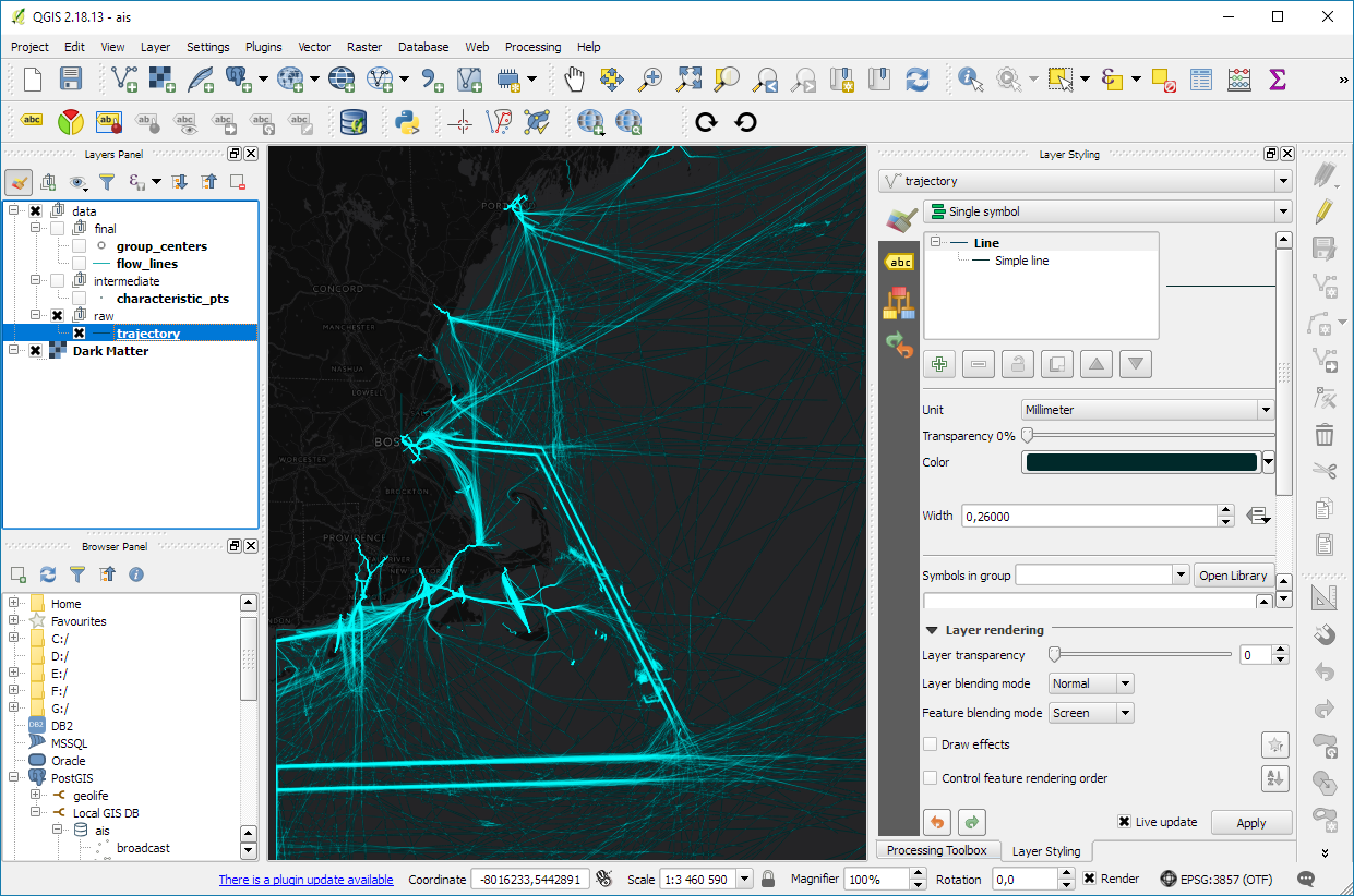
There are multiple ways to model trajectory data. This post takes a closer look at the OGC® Moving Features Encoding Extension: Simple Comma Separated Values (CSV). This standard has been published in 2015 but I haven’t been able to find any reviews of the standard (in a GIS context or anywhere else).

The following analysis is based on the official OGC trajcectory example at http://docs.opengeospatial.org/is/14-084r2/14-084r2.html#42. The header consists of two lines: the first line provides some meta information while the second defines the CSV columns. The data model is segment based. That is, each line describes a trajectory segment with at least two coordinate pairs (or triplets for 3D trajectories). For each segment, there is a start and an end time which can be specified as absolute or relative (offset) values:

@stboundedby,urn:x-ogc:def:crs:EPSG:6.6:4326,2D,50.23 9.23,50.31 9.27,2012-01-17T12:33:41Z,2012-01-17T12:37:00Z,sec
@columns,mfidref,trajectory,state,xsd:token,”type code”,xsd:integer
a, 10,150,11.0 2.0 12.0 3.0,walking,1
b, 10,190,10.0 2.0 11.0 3.0,walking,2
a,150,190,12.0 3.0 10.0 3.0,walking,2
c, 10,190,12.0 1.0 10.0 2.0 11.0 3.0,vehicle,1

Let’s look at the first data row in detail:

  • a … trajectory id
  • 10 … start time offset from 2012-01-17T12:33:41Z in seconds
  • 150 … end time offset from 2012-01-17T12:33:41Z in seconds
  • 11.0 2.0 12.0 3.0 … trajectory coordinates: x1, y1, x2, y2
  • walking …  state
  • 1… type code

My main issues with this approach are

  1. They missed the chance to use WKT notation to make the CSV easily readable by existing GIS tools.
  2. As far as I can see, the data model requires a regular sampling interval because there is no way to store time stamps for intermediate positions along trajectory segments. (Irregular intervals can be stored using segments for each pair of consecutive locations.)

In the common GIS simple feature data model (which is point-based), the same data would look something like this:

traj_id,x,y,t,state,type_code
a,11.0,2.0,2012-01-17T12:33:51Z,walking,1
a,12.0,3.0,2012-01-17T12:36:11Z,walking,1
a,10.0,3.0,2012-01-17T12:36:51Z,walking,2
b,10.0,2.0,2012-01-17T12:33:51Z,walking,2
b,11.0,3.0,2012-01-17T12:36:51Z,walking,2
c,12.0,1.0,2012-01-17T12:33:51Z,vehicle,1
c,10.0,2.0,2012-01-17T12:35:21Z,vehicle,1
c,11.0,3.0,2012-01-17T12:36:51Z,vehicle,1

The main issue here is that there has to be some application logic that knows how to translate from points to trajectory. For example, trajectory a changes from walking1 to walking2 at 2012-01-17T12:36:11Z but we have to decide whether to store the previous or the following state code for this individual point.

An alternative to the common simple feature model is the PostGIS trajectory data model (which is LineStringM-based). For this data model, we need to convert time stamps to numeric values, e.g. 2012-01-17T12:33:41Z is 1326803621 in Unix time. In this data model, the data looks like this:

traj_id,trajectory,state,type_code
a,LINESTRINGM(11.0 2.0 1326803631, 12.0 3.0 1326803771),walking,1
a,LINESTRINGM(12.0 3.0 1326803771, 10.0 3.0 1326803811),walking,2
b,LINESTRINGM(10.0 2.0 1326803631, 11.0 3.0 1326803811),walking,2
c,LINESTRINGM(12.0 1.0 1326803631, 10.0 2.0 1326803771, 11.0 3.0 1326803811),vehicle,1

This is very similar to the OGC data model, with the notable difference that every position is time-stamped (instead of just having segment start and end times). If one has movement data which is recorded at regular intervals, the OGC data model can be a bit more compact, but if the trajectories are sampled at irregular intervals, each point pair will have to be modeled as a separate segment.

Since the PostGIS data model is flexible, explicit, and comes with existing GIS tool support, it’s my clear favorite.


Read more:

Movement data in GIS extra: trajectory generalization code and sample data

Today’s post is a follow-up of Movement data in GIS #3: visualizing massive trajectory datasets. In that post, I summarized a concept for trajectory generalization. Now, I have published the scripts and sample data in my QGIS-Processing-tools repository on Github.

To add the trajectory generalization scripts to your Processing toolbox, you can use the Add scripts from files tool:

It is worth noting, that Add scripts from files fails to correctly import potential help files for the scripts but that’s not an issue this time around, since I haven’t gotten around to actually write help files yet.

The scripts are used in the following order:

  1. Extract characteristic trajectory points
  2. Group points in space
  3. Compute flows between cells from trajectories

The sample project contains input data, as well as output layers of the individual tools. The only required input is a layer of trajectories, where trajectories have to be LINESTRINGM (note the M!) features:

Trajectory sample based on data provided by the GeoLife project

In Extract characteristic trajectory points, distance parameters are specified in meters, stop duration in seconds, and angles in degrees. The characteristic points contain start and end locations, as well as turns and stop locations:

The characteristic points are then clustered. In this tool, the distance has to be specified in layer units, which are degrees in case of the sample data.

Finally, we can compute flows between cells defined by these clusters:

Flow lines scaled by flow strength and cell centers scaled by counts

If you use these tools on your own data, I’d be happy so see what you come up with!


Read more:

Movement data in GIS #6: updates from AGILE2017

AGILE 2017 is the annual international conference on Geographic Information Science of the Association of Geographic Information Laboratories in Europe (AGILE) which was established in 1998 to promote academic teaching and research on GIS.

This years conference in Wageningen was my time at AGILE.  I had the honor to present our recent work on pedestrian navigation with landmarks [Graser, 2017].

If you are interested in trying it, there is an online demo. The conference also provided numerous pointers toward ideas for future improvements, including [Götze and Boye, 2016] and [Du et al., 2017]

On the issue of movement data in GIS, there weren’t too many talks on this topic at AGILE but on the conceptual side, I really enjoyed David Jonietz’ talk on how to describe trajectory processing steps:

Source: [Jonietz and Bucher, 2017]

In the pre-conference workshop I attended, there was also an interesting presentation on analyzing trajectory data with PostGIS by Phd candidate Meihan Jin.

I’m also looking forward to reading [Wiratma et al., 2017] “On Measures for Groups of Trajectories” because I think that the presentation only scratched the surface.

References

[Du et al, 2017] Du, S., Wang, X., Feng, C. C., & Zhang, X. (2017). Classifying natural-language spatial relation terms with random forest algorithm. International Journal of Geographical Information Science, 31(3), 542-568.
[Götze and Boye, 2016] Götze, J., & Boye, J. (2016). Learning landmark salience models from users’ route instructions. Journal of Location Based Services, 10(1), 47-63.
[Graser, 2017] Graser, A. (2017). Towards landmark-based instructions for pedestrian navigation systems using OpenStreetMap, AGILE2017, Wageningen, Netherlands.
[Jonietz and Bucher, 2017] Jonietz, D., Bucher, D. (2017). Towards an Analytical Framework for Enriching Movement Trajectories with Spatio-Temporal Context Data, AGILE2017, Wageningen, Netherlands.
[Wiratma et al., 2017] Wiratma L., van Kreveld M., Löffler M. (2017) On Measures for Groups of Trajectories. In: Bregt A., Sarjakoski T., van Lammeren R., Rip F. (eds) Societal Geo-innovation. GIScience 2017. Lecture Notes in Geoinformation and Cartography. Springer, Cham


  • Page 1 of 1 ( 5 posts )
  • trajectories

Back to Top

Sustaining Members