Related Plugins and Tags

QGIS Planet

Native point cloud processing in QGIS

After the addition of support for visualising point clouds in the recent versions of QGIS, the next step was to add the processing tools so users can manage and analyse their data.

There are several 3rd party QGIS plugins (either proprietary or not fully open source) which allow users to interrogate and analyse lidar data. But with our latest work, we have introduced powerful point cloud algorithms to the QGIS Processing framework. All the algorithms are available out of the box in QGIS 3.32, with no need to install plugins.

In this blog post, we summarise the initial point cloud algorithms for QGIS Processing toolbox which will be available in QGIS 3.32 (to be released at the end of June 2023). This work was made possible by the generous donations to our crowdfunding.

Point Cloud algorithms in QGIS

First off a quick look at the new algorithms as shown in the Processing toolbox in three groups:
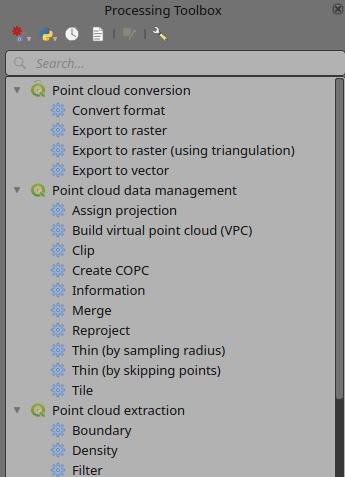
Point Cloud algorithms in QGIS processing toolbox

Point Cloud algorithms in QGIS processing toolbox
  • Convert formats: this will allow you to convert your point cloud data between LAS and LAZ formats for the time being. Other PDAL supported formats can be added later.
  • Export to raster: with this algorithm you can export point cloud to a regularly gridded raster data. It uses inverse distance weighting to assign raster cell values. Raster cells with no nearby points will get “no data” values (these holes may be removed by using “Fill nodata” raster algorithm).
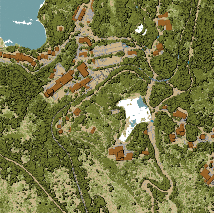
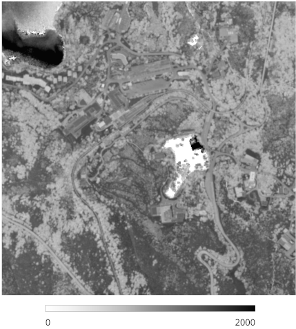
Input point cloud layer file

Input point cloud layer file

Raster output using Intensity attribute of points

Raster output using Intensity attribute of points
  • Export to raster (using triangulation): this allows you to export Z data to a regularly gridded raster by interpolating between the points using triangulation. Note that this can be slower if you are dealing with a large dataset. If your point cloud is dense, you can export your ground points as a raster using the Export to raster algorithm.
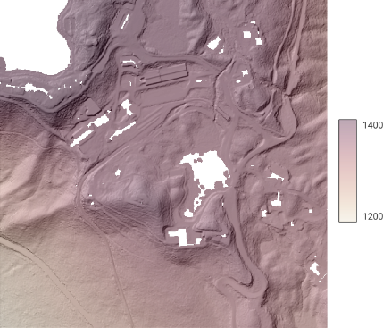
Terrain raster output generated by point cloud triangulation

Terrain raster output generated by point cloud triangulation
  • Export to vector: to export point cloud to other vector formats. This is useful to export some of your data for software applications which do not support point cloud data and still use formats such as CSV, Shapefile, DXF.
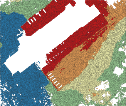
Exporting point cloud (ground points) to Shapefile styled based on the elevation

Exporting point cloud (ground points) to Shapefile styled based on the elevation!
  • Assign projection: assigns a projection to a point cloud layer (if it is wrong or missing)
  • Build virtual point cloud (VPC): with this algorithm you can generate a virtual file (based on STAC specification) and load them as a single file in QGIS. There will be a separate blog post detailing this new exciting feature.
  • Clip: clip a point cloud layer by a vector polygon layer.
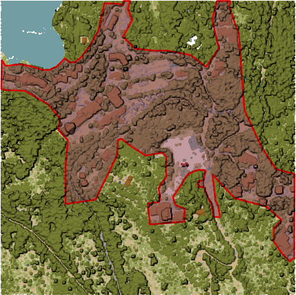
Input point cloud layer and a polygon coverage

Input point cloud layer and a polygon coverage

Result of the clipping algorithm

Result of the clipping algorithm
  • Create COPC: when you load a non-indexed point cloud layer in QGIS, it will take a while for the application to create the COPC index for your file. With this algorithm, you can create the index for all your files in a batch mode.
  • Information: displays information from a point cloud layer:
LAS           1.4
point format  6
count         56736130
scale         0.001 0.001 0.001
offset        431749.999 5440919.999 968.898
extent        431250 5440420 424.266
              432249.999 5441419.999 1513.531
crs           ETRS89 / UTM zone 34N (N-E) (EPSG:3046)  (vertical CRS missing!)
units         horizontal=metre  vertical=unknown

Attributes:
 - X floating 8
 - Y floating 8
 - Z floating 8
 - Intensity unsigned 2
 - ReturnNumber unsigned 1
 - NumberOfReturns unsigned 1
 - ScanDirectionFlag unsigned 1
 - EdgeOfFlightLine unsigned 1
 - Classification unsigned 1
 - ScanAngleRank floating 4
 - UserData unsigned 1
 - PointSourceId unsigned 2
 - GpsTime floating 8
 - ScanChannel unsigned 1
 - ClassFlags unsigned 1

Output from point cloud information algorithm

  • Merge: join multiple point cloud layers into a single file
  • Reproject: reproject the input file to a different coordinate reference system
  • Thin (by sampling radius): reduces the number of points within a certain radius
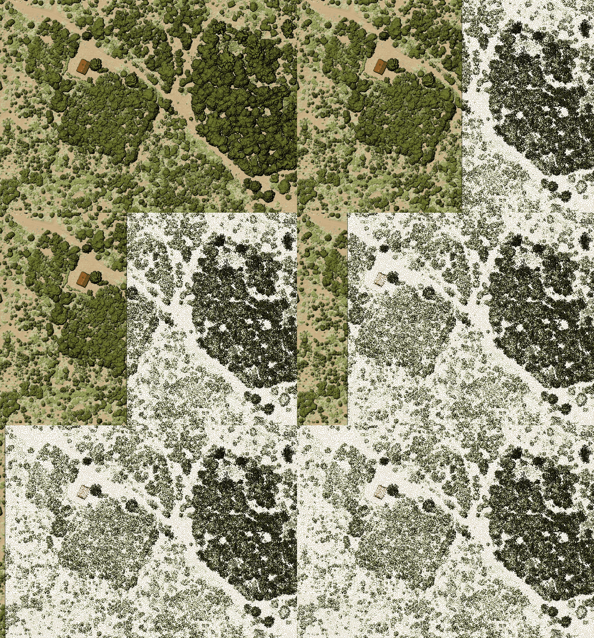
Thining point cloud (by sampling radius)

Thining point cloud (by sampling radius)
  • Thin (by skipping points): reduces the number of points by skipping nearby points
  • Tile: this algorithm generates a set of tiles based on the input point cloud layer and tile size
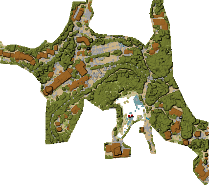
  • Boundary: generates a (multi) polygon from your point cloud data. The output file might contain holes depending on the density of your point cloud input data.
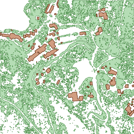
Extracting high vegetation and building polygons from an input point cloud layer

Extracting high vegetation and building polygons from an input point cloud layer
  • Density: outputs a raster file based on the number of points within each raster cell - useful for quality checking of point cloud datasets
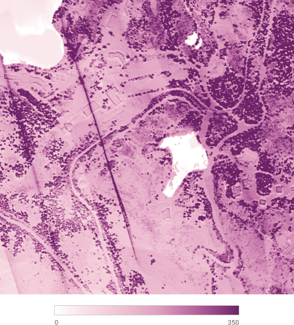
Point density (number of points per 2x2 m)  as a raster

Point density (number of points per 2x2 m) as a raster
  • Filter: it creates a new file based on the filter set as an expression. Note that most of the algorithms support on-the-fly filtering under the Advanced parameters.
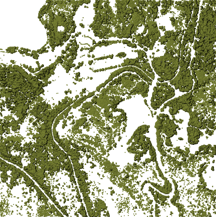
Filtering of high vegetation class from an input point cloud layer

Filtering of high vegetation class from an input point cloud layer

Behind the scenes

All the heavy lifting of the point cloud processing is done by PDAL - a state of the art open source library for processing point clouds. PDAL provides a wide range of “readers”, “filters” and “writers” to build complex pipelines to process point clouds.

We have built a new standalone command line tool pdal_wrench on top of PDAL. It addresses two major issues that non-expert users typically face when working with PDAL:

  • Ease of use: not everyone finds it easy to manually craft JSON files with pipelines, study manuals of the many stages and read details about file formats involved.
  • Parallel execution: PDAL runs pipelines in a single thread, so only one CPU gets to do the work normally and users need to implement their own parallelism if they want to speed up processing.

The command line tool provides a simple set of commands that take care of everything. For example, to export a raster layer with elevations (DEM) with 1 meter resolution:

pdal_wrench to_raster --output=raster.tif --resolution=1 --attribute=Z data.las

The pdal_wrench tool does not depend on QGIS, so it can be easily used separately.

The commands are designed to run in parallel when there are multiple input files or when the input file is in COPC format. Depending on the algorithm, the work gets split spatially into square tiles (1000x1000 map units by default) for parallel processing, or individual files are processed in parallel. With a single ordinary LAS/LAZ file on input, there is currently no parallelism going on.

For commands that are sensitive to edge artifacts (such as export to raster), we take care of processing extra points outside of the extent of each tile (referred to as collar or buffer) to make sure the results are correct as if no tiling would be happening (see Martin Isenburg’s article for more details: https://rapidlasso.com/2015/08/07/use-buffers-when-processing-lidar-in-tiles/).

Future work

The current list of point cloud algorithms already allows users to do plenty of work. But more could be added to the toolbox - algorithms that are already supported by PDAL, but not exposed in QGIS: classification, noise removal, surface reconstruction, clustering, height above ground, colorizing and many more. If you are interested in more point cloud processing algorithms in QGIS, please contact us and we will be happy to add them to future QGIS releases.

SLYR Update — June 2023

Welcome back, SLYR enthusiasts! We’re thrilled to share the latest updates and enhancements for our SLYR ESRI to QGIS Compatibility Suite that will dramatically streamline the use of ESRI documents within QGIS (and vice versa!). Our team has been hard at work, expanding the capabilities of SLYR to ensure seamless compatibility between the latest QGIS and ArcGIS releases. We’ve also got some exciting news for users of the Community Edition of SLYR! Let’s dive right in and explore the exciting new features that have been added to SLYR since our previous update

Converting Raster Layers in Geodatabases

We’re pleased to announce that SLYR now offers support for converting raster layers within Geodatabases. With this update, users can effortlessly migrate their raster data from ESRI’s Geodatabases to QGIS, enabling more efficient data management and analysis.

This enhancement is only possible thanks to work in the fantastic GDAL library which underpins QGIS’ raster data support. Please ensure that you have the latest version of QGIS (3.30.3 or 3.28.7 at a minimum) to make the most of this feature.

Annotation and Graphic Layer Improvements

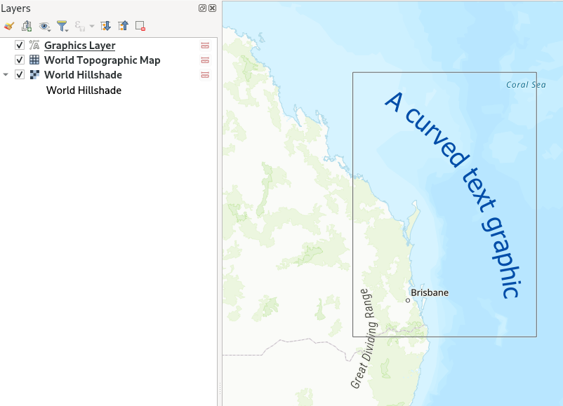
Text Annotations along Curves

For those working with curved annotations, we’ve got you covered! SLYR now supports the conversion of text annotations along curves in QGIS. With this enhancement, you’ll get accurate conversion of any curved text and text-along-line annotations from MXD and APRX documents. This has been a long-requested feature which we can now introduce thanks to enhancements coming in QGIS 3.32.

ArcGIS Pro Graphics Layer Support

SLYR now supports the conversion of ArcGIS Pro graphics layers, converting all graphic elements to their QGIS “Annotation Layer” equivalents. If you’ve spent hours carefully designing cartographic markup on your maps, you can be sure that SLYR will allow you to re-use this work within QGIS!

Curved text graphic conversion

Enhanced Page Layout Support

We’ve further improved the results of converting ArcGIS Pro page layouts to QGIS print layouts, with dozens of refinements to the conversion results. The highlights here include:

  • Support for converting measured grids and graticules to QGIS map grids
  • Enhanced dynamic text conversions:  Now, when migrating your projects, you can expect a smoother transition for dynamic text ensuring your layouts correctly show generated metadata and text correctly
  • Support for north arrows, grouped elements, legends and table frames.

Rest assured that your carefully crafted map layouts will retain their visual appeal and functionality when transitioning to QGIS!

Improved QGIS to ArcGIS Pro Conversions

SVG Marker Exports and Symbology Size

SLYR has introduced initial support for exporting SVG markers from QGIS to ArcGIS Pro formats. SVG graphics are a component of QGIS’ cartography, and are frequently used to create custom marker symbols. Unfortunately, ArcGIS Pro doesn’t have any native support for SVG graphics for marker symbols, instead relying on a one-off conversion from SVG to multiple separate marker graphics whenever an SVG is imported into ArcGIS Pro. Accordingly, we’ve implemented a similar logic in SLYR in order to convert SVG graphics to ArcGIS Pro marker graphics transparently whenever QGIS symbology is exported to ArcGIS. This enhancement allows for a seamless transfer of symbology from QGIS, ensuring that your converted maps retain their visual integrity.

Furthermore, the update includes support for exporting QGIS symbology sizes based on “map unit” measurements to ArcGIS Pro, resulting in ArcGIS Pro symbology which more accurately matches the original QGIS versions.

Rule-Based Renderer Conversion

The “Rule Based Renderer” is QGIS’ ultimate powerhouse for advanced layer styling. It’s extremely flexible, thanks to its support for nested rules and filtering using QGIS expressions. However, this flexibility comes with a cost — there’s just no way to reproduce the same results within ArcGIS Pro’s symbology options! Newer SLYR releases will now attempt to work around this by implementing basic conversion of QGIS rule-based renderers to ArcGIS Pro layers with “display filters” attached. This allows us to convert some basic rule-based configuration to ArcGIS Pro formats.

There’s some limitations to be aware of:

  1. Only “flat” rule structures can be converted. It’s not possible to convert a nested rule structure into something representable by ArcGIS Pro.
  2. While the QGIS expression language is very rich and offers hundreds of functions for use in expressions, only basic QGIS filter expressions can be converted to ArcGIS Pro rules.

Improved Conversion of Raster and Mesh Layers

Based on user feedback, we’ve made significant improvements to the conversion of QGIS rasters and mesh layers to ArcGIS Pro formats. Expect enhanced accuracy when migrating these types of data, ensuring a closer match between your QGIS projects and their ArcGIS Pro equivalents.

New tools

The latest SLYR release introduces some brand new tools for automating your conversion workflows:

Convert LYR/LYRX Files Directly to SLD

To facilitate interoperability, SLYR has introduced algorithms that directly convert ESRI LYR or LYRX files to the “SLD” format (Styled Layer Descriptor). This feature simplifies the process of sharing and utilizing symbology between different GIS software, allowing for direct conversion of ESRI symbology for use in Geoserver or Mapserver.

Convert File Geodatabases to Geopackage

We’re thrilled to introduce a powerful new tool in SLYR that enables a comprehensive conversion of a File Geodatabase to the Geopackage format. With this feature, you can seamlessly migrate your data from ESRI’s File Geodatabase format to the versatile and widely supported GeoPackage format. As well as the raw data conversion, this tool also ensures the conversion of field domains and other advanced Geodatabase functionality to their GeoPackage equivalent, preserving valuable metadata and maintaining data integrity throughout the transition. (Please note that this tool requires QGIS version 3.28 or later.)


All these exciting additions to SLYR are available today to SLYR license holders. If you’re after one-click, accurate conversion of projects from ESRI to QGIS, contact us to discuss your licensing needs.

As described on our SLYR page, we also provide some of the conversion tools for free use via the SLYR “Community Edition”. We’re proud to announce that we’ve just hit the next milestone in the Community Edition funding, and will now be releasing all of SLYR’s support for raster LYR files to the community edition! This complements the existing support for vector LYR files and ESRI style files available in the community edition. For more details on the differences between the licensed and community editions, see our product comparison.

QField 2.8: Boosting field work through external sensors

The latest version of QField is out, featuring as its main new feature sensor handling alongside the usual round of user experience and stability improvements. We simply can’t wait to see the sensor uses you will come up with!

The main highlight: sensors

QField 2.8 ships with out-of-the-box handling of external sensor streams over TCP, UDP, and serial port. The functionality allows for data captured through instruments – such as geiger counter, decibel sensor, CO detector, etc. – to be visualized and manipulated within QField itself.

Things get really interesting when sensor data is utilized as default values alongside positioning during the digitizing of features. You are always one tap away from adding a point locked onto your current position with spatially paired sensor readings saved as point attribute(s).

Not wowed yet? Try pairing sensor readings with QField’s tracking capability! 😉 Head over QField’s documentation on this as well as QGIS’ section on sensor management to know more.

The development of this feature involved the addition of a sensor framework in upstream QGIS which will be available by the end of this coming June as part of the 3.32 release. This is a great example of the synergy between QField and its big brother QGIS, whereas development of new functionality often benefits the broader QGIS community. Big thanks to Sevenson Environmental Services for sponsoring this exciting capability.

Notable improvements

A couple of refinements during this development cycle are worth mentioning. If you ever wished for QField to directly open a selected project or reloading the last session on app launch, you’ll be happy to know this is now possible.

For heavy users of value relations in their feature forms, QField is now a tiny bit more clever when displaying string searches against long lists, placing hits that begin with the matched string first as well as visually highlighting matches within the result list itself.

Finally, feature lists throughout QField are now sorted. By default, it will sort by the display field or expression defined for each vector layer, unless an advanced sorting has been defined in a given vector layer’s attribute table. It makes browsing through lists feel that much more natural.

2.8.1 - Insightful Indri

Changes

🐛 Bug Fixes

  • Insure layer visibility is always properly reflected in the legend widget
  • Fix checkbox editor widget not reflecting feature values
  • Fix default value when tracking against point layers
  • Fix HTML code in HTML-enabled multiline text editor widget

Analyzing video-based bicycle trajectories

Did you know that MovingPandas also supports local image coordinates? Indeed, it does.

In today’s post, we will explore how we can use this feature to analyze bicycle tracks extracted from video footage published by Michael Szell @mszll:

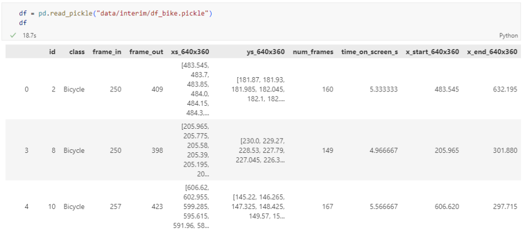
The bicycle trajectory coordinates are stored in two separate lists: xs_640x360 and ys640x360:

This format is kind of similar to the Kaggle Taxi dataset, we worked with in the previous post. However, to use the solution we implemented there, we need to combine the x and y coordinates into nice (x,y) tuples:

df['coordinates'] = df.apply(
    lambda row: list(zip(row['xs_640x360'], row['ys_640x360'])), axis=1)
df.drop(columns=['xs_640x360', 'ys_640x360'], inplace=True)

Afterwards, we can create the points and compute the proper timestamps from the frame numbers:

def compute_datetime(row):
    # some educated guessing going on here: the paper states that the video covers 2021-06-09 07:00-08:00
    d = datetime(2021,6,9,7,0,0) + (row['frame_in'] + row['running_number']) * timedelta(seconds=2)
    return d
def create_point(xy):
    try: 
        return Point(xy)
    except TypeError:  # when there are nan values in the input data
        return None
new_df = df.head().explode('coordinates')
new_df['geometry'] = new_df['coordinates'].apply(create_point)
new_df['running_number'] = new_df.groupby('id').cumcount()
new_df['datetime'] = new_df.apply(compute_datetime, axis=1)
new_df.drop(columns=['coordinates', 'frame_in', 'running_number'], inplace=True)
new_df

Once the points and timestamps are ready, we can create the MovingPandas TrajectoryCollection. Note how we explicitly state that there is no CRS for this dataset (crs=None):

trajs = mpd.TrajectoryCollection(
    gpd.GeoDataFrame(new_df), 
    traj_id_col='id',  t='datetime', crs=None)

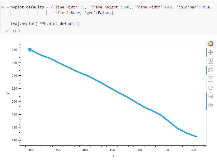
Plotting trajectories with image coordinates

Similarly, to plot these trajectories, we should tell hvplot that it should not fetch any background map tiles (’tiles’:None) and that the coordinates are not geographic (‘geo’:False):

If you want to explore the full source code, you can find my Github fork with the Jupyter notebook at: https://github.com/anitagraser/desirelines/blob/main/mpd.ipynb

The repository also contains a camera image of the intersection, which we can use as a background for our trajectory plots:

bg_img = hv.RGB.load_image('img/intersection2.png', bounds=(0,0,640,360)) 

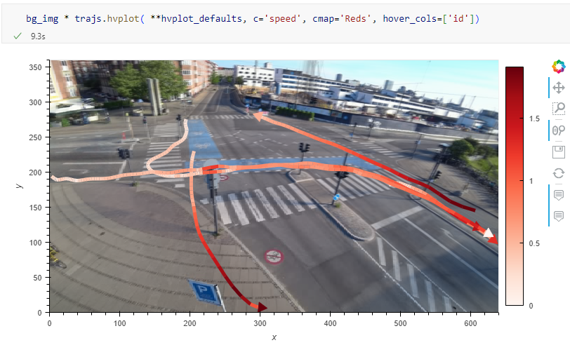
One important caveat is that speed will be calculated in pixels per second. So when we plot the bicycle speed, the segments closer to the camera will appear faster than the segments in the background:

To fix this issue, we would have to correct for the distortions of the camera lens and perspective. I’m sure that there is specialized software for this task but, for the purpose of this post, I’m going to grab the opportunity to finally test out the VectorBender plugin.

Georeferencing the trajectories using QGIS VectorBender plugin

Let’s load the five test trajectories and the camera image to QGIS. To make sure that they align properly, both are set to the same CRS and I’ve created the following basic world file for the camera image:

1
0
0
-1
0
360

Then we can use the VectorBender tools to georeference the trajectories by linking locations from the camera image to locations on aerial images. You can see the whole process in action here:

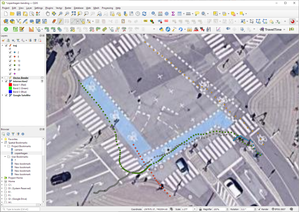
After around 15 minutes linking control points, VectorBender comes up with the following georeferenced trajectory result:

Not bad for a quick-and-dirty hack. Some points on the borders of the image could not be georeferenced since I wasn’t always able to identify suitable control points at the camera image borders. So it won’t be perfect but should improve speed estimates.


This post is part of a series. Read more about movement data in GIS.

How to use Kaggle’s Taxi Trajectory Data in MovingPandas

Kaggle’s “Taxi Trajectory Data from ECML/PKDD 15: Taxi Trip Time Prediction (II) Competition” is one of the most used mobility / vehicle trajectory datasets in computer science. However, in contrast to other similar datasets, Kaggle’s taxi trajectories are provided in a format that is not readily usable in MovingPandas since the spatiotemporal information is provided as:

  • TIMESTAMP: (integer) Unix Timestamp (in seconds). It identifies the trip’s start;
  • POLYLINE: (String): It contains a list of GPS coordinates (i.e. WGS84 format) mapped as a string. The beginning and the end of the string are identified with brackets (i.e. [ and ], respectively). Each pair of coordinates is also identified by the same brackets as [LONGITUDE, LATITUDE]. This list contains one pair of coordinates for each 15 seconds of trip. The last list item corresponds to the trip’s destination while the first one represents its start;

Therefore, we need to create a DataFrame with one point + timestamp per row before we can use MovingPandas to create Trajectories and analyze them.

But first things first. Let’s download the dataset:

import datetime
import pandas as pd
import geopandas as gpd
import movingpandas as mpd
import opendatasets as od
from os.path import exists
from shapely.geometry import Point

input_file_path = 'taxi-trajectory/train.csv'

def get_porto_taxi_from_kaggle():
    if not exists(input_file_path):
        od.download("https://www.kaggle.com/datasets/crailtap/taxi-trajectory")

get_porto_taxi_from_kaggle()
df = pd.read_csv(input_file_path, nrows=10, usecols=['TRIP_ID', 'TAXI_ID', 'TIMESTAMP', 'MISSING_DATA', 'POLYLINE'])
df.POLYLINE = df.POLYLINE.apply(eval)  # string to list
df

And now for the remodelling:

def unixtime_to_datetime(unix_time):
    return datetime.datetime.fromtimestamp(unix_time)

def compute_datetime(row):
    unix_time = row['TIMESTAMP']
    offset = row['running_number'] * datetime.timedelta(seconds=15)
    return unixtime_to_datetime(unix_time) + offset

def create_point(xy):
    try: 
        return Point(xy)
    except TypeError:  # when there are nan values in the input data
        return None
 
new_df = df.explode('POLYLINE')
new_df['geometry'] = new_df['POLYLINE'].apply(create_point)
new_df['running_number'] = new_df.groupby('TRIP_ID').cumcount()
new_df['datetime'] = new_df.apply(compute_datetime, axis=1)
new_df.drop(columns=['POLYLINE', 'TIMESTAMP', 'running_number'], inplace=True)
new_df

And that’s it. Now we can create the trajectories:

trajs = mpd.TrajectoryCollection(
    gpd.GeoDataFrame(new_df, crs=4326), 
    traj_id_col='TRIP_ID', obj_id_col='TAXI_ID', t='datetime')
trajs.hvplot(title='Kaggle Taxi Trajectory Data', tiles='CartoLight')

That’s it. Now our MovingPandas.TrajectoryCollection is ready for further analysis.

By the way, the plot above illustrates a new feature in the recent MovingPandas 0.16 release which, among other features, introduced plots with arrow markers that show the movement direction. Other new features include a completely new custom distance, speed, and acceleration unit support. This means that, for example, instead of always getting speed in meters per second, you can now specify your desired output units, including km/h, mph, or nm/h (knots).


This post is part of a series. Read more about movement data in GIS.

Plugin Update April 2023

April wasn’t just the month of our wonderful user conference and contributor meeting, it was also a month with a whopping 23 new plugins that have been published in the QGIS plugin repository.

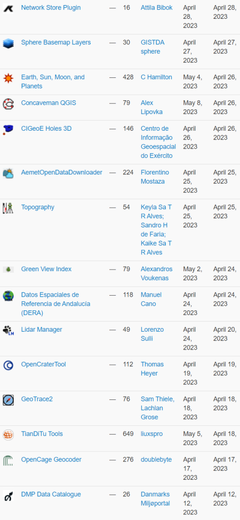
Here’s the quick overview in reverse chronological order. If any of the names or short descriptions piques your interest, you can find the direct link to the plugin page in the table below the screenshot.

Network Store Plugin
export layers to kisters network store
Sphere Basemap Layers
This plugin let you to add a variety of thailand basemap from GISTDA sphere Open Platform
Earth, Sun, Moon, and Planets
Tools to calculate the positions of the sun, moon, and planets when viewed from directly overhead for a particular date and time. It displays solar and lunar information for a coordinate at the specified date and time. (Note the Python library dependencies.)
Concaveman QGIS
Makes concave hull for points
CIGeoE Holes 3D
Draws holes in polygons (3D)
AemetOpenDataDownloader
This Plugin download open data from aemet
Topography
The plugin is available in this first version with the functionality to calculate closed polygons using the projections method.
Green View Index
A plugin for Green View Index (GVI) operations
Datos Espaciales de Referencia de Andalucía (DERA)
Loading of wfs/wms services from DERA Spatial Reference Data.Carga de los servicios wfs/wms de los Datos Espaciales de Referencia DERA
Lidar Manager
Manage LiDAR (dtm/dsm) dataset from Tile Index Layer
OpenCraterTool
A tool to measure and compare craters
GeoTrace2
A QGIS plugin for geological mapping
TianDiTu Tools
天地图底图加载
OpenCage Geocoder
Geocoding using the OpenCage API
DMP Data Catalogue
Discover and add layers from the Danish Miljøportal data catalog
File Management
Plugin to help with file management from the Layers Panel.
Bestagon
Form (mostly Hexagon) generator for point intensities
Indiana Ortho Imagery
This plugin provide easy access to Indiana Ortho Imageries
Adresssuche
Searching for an adresspoint in Germany based on offical data – ALKIS Adresssuche
GpuDataChecker
Plugin pour l’aide au contrôle de la validité géométrique de données pour intégration dans le géoportail de l’urbanisme
Tile Index Generator
This plugin creates tile index in vector format for XYZ tiles.
SeaLevelTool
Adjust styling on raster layer by a sea level curve.
DataSud
Plugin pour QGIS 3 fournissant un accès simple aux flux de données géographiques (WMS, WFS) publiées par la Région Sud sur DataSud.fr.

(Nederlands) Communicatie is een beetje… lastig?

Sorry, this entry is only available in Dutch.

Integrate a QGIS Cloud Map into a Web Page

After a beautiful map has been created with QGIS and published on https://qgiscloud.com, the desire quickly arises to integrate this map into one’s own website. This way, visitors to the website could access the map directly and without having to go via https://qgiscloud.com. With a little HTML, this is easy to do. But let’s start from the beginning. Make a QGIS Cloud Map As always with QGIS Cloud, a map must first be published.

QGIS UC 2023, ‘s-Hertogenbosch

Sorry… no English text as of yet. However, you’re welcome to have a look at the Dutch version (and use some automagic translation device)…

Reporting Back From the User Conference & Contributor Meeting in Den Bosch

Last week, we had our 25th Contributor Meeting in ‘s-Hertogenbosch, The Netherlands. Prior to the meeting, the International QGIS User Conference, brought together 200 participants from all around the world who came to learn about QGIS and exchange ideas and best practices.

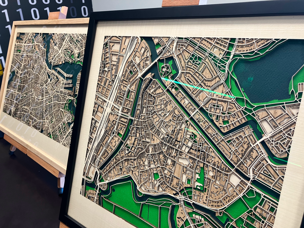
The conference programme was jam-packed with great content. Over 50 presentations were given during the conference, with the participants enjoying the Dutch atmosphere whilst building up their knowledge of QGIS and sharing their ideas. With more than 20 years of development behind us, QGIS has become a stable platform that supports geospatial decision making, analysis and decision making in all sorts of endeavours. We saw lots of talks that demonstrated this maturity, for example a presentation John Holden and Blake Esselsteyn showed how QGIS is being used to determine voting districts to support the democratic process, Angelina Savchuk showed how QGIS is being used to support the work of the Red Cross, whilst Nick Vervaal showed us how QGIS is used to make high tech artistic laser cut maps from wood.

We were honoured to be joined by Lucho Ferrer who came all the way from Peru! Ujaval Gandhi travelled all the way from India and wowed the audience with his workshop on QGIS Actions.

There are two mobile offerings for QGIS users who want to take their work out to the field. Both QField and MerginMaps had a strong presence at the User Conference, causing a lot of excitement and buzz in the audience.

Contributor Meeting

As is traditional, the contributor meeting (which was held directly after the two day user conference) was full of workshops, sessions, and spontaneous get-togethers to facilitate the exchange between community members, including sessions on:

  • Onboarding Day
  • Plans for the certification programme
  • Getting around in the QGIS community
  • Translating QGIS 
  • Documentation system and process
  • Editing the documentation online on GitHub
  • Building documentation on your local machine and using Git to make a pull request (submission)
  • Compiling QGIS
  • Making your first pull request to QGIS
  • Create QGIS issues and feature requests
  • OGC API in QGIS
  • QGIS vision
  • QGIS website update
Everyone worked hard to advance the project, the open plan space facilitating lots of ad hoc conversations which are hard to match in an online environment.
OGC API in QGIS: current support and proposed developments, hosted by Joana Simoes

From the QGIS community we would like to extend a huge ‘thank you!’ to the local organising team who hosted a flawless event and worked so hard to make sure everyone had the best experience possible. Thank you and see you next year!

2.7.6 - Heroic Hedgehog

Changes

🐛 Bug Fixes

  • Yet more bug fixing and stability improvements.

2.7.5 - Heroic Hedgehog

Changes

🐛 Bug Fixes

  • More bug fixing and stability improvements.

2.7.4 - Heroic Hedgehog

Changes

🐛 Bug Fixes

  • Many, many fixes.

QGIS Grants #8: Call for Grant Proposals 2023

Dear QGIS Community,

We are very pleased to announce that this year’s round of grants is now available. The call is open to anybody who wants to make a contribution to QGIS funded by our grant fund, subject to the call conditions outlined in the application form.

The deadline for this round is in four weeks, on 2nd May 2023.

There are no new procedures in 2023. Please note the following guidelines established in previous years: 

  • The proposal must be submitted as a ‘QEP’ (QGIS Enhancement Proposal) issue in the repo: https://github.com/qgis/QGIS-Enhancement-Proposals (tagged as Grant-YEAR). Following this approach will allow people to ask questions and provide public feedback on individual proposals.
  • Proposals must clearly define the expected final result so that we can properly assess if the goal of the proposal has been reached.
  • The project budgets should account for PR reviewing expenses to ensure timely handling of the project-related PRs and avoid delays caused by relying on reviewer volunteer time. 
  • In the week after the QEP discussion period, the proposal authors are expected to write a short summary of the discussion that is suitable for use as a basis on which voting members make their decisions. 

The PSC of QGIS.ORG will examine the proposals and has veto power in case a proposal does not follow guidelines or is not in line with project priorities.

For more details, please read the introduction provided in the application form.

We look forward to seeing all your great ideas for improving QGIS!

Capturing more while in the field with the new QField 2.7

A brand new version of QField has been released, packed with features that will make you fall in love with this essential open source tool all over again with a focus on capturing more while you are in the field. QField 2.7 nicknamed “Heroic Hedgehog” also includes a number of worthy fixes making it a crucial update to get.

New recording capabilities

The highlight of QField 2.7 is the new audio and video recording capability straight from the feature form. In addition to preexisting still photo capture, this functionality allows for video motion and audio clips to be added as attachments to feature attributes.

The audio recording capability can come in handy in the field when typing on a keyboard-less device can be challenging. Simply record an audio note of observations to process later.

The experience wouldn’t be complete without audio and video playback support, which we took care of in this version too. Playback of such media content within the feature form gives an immediate feedback and saves time. For those interested in full screen immersion, simply click on the video frame to open the attached in your favorite media player. We also took the opportunity to implement audio and video playback on QGIS so people can easily consume the fruits of their labor in the field at their workstation.

We would be remiss if we didn’t mention map canvas rotation functionality added in this version. This is a long-requested functionality which we are happy to have packed into QField now. Pro-tip: when positioning is enabled, double tapping on the lower-left positioning button will have the map canvas follow both the device’s current location as well as the compass orientation.

Finally – some would argue “most importantly” 😉 – QField is now equipped with a beautiful dark theme which users can activate in the settings panel. By default on Android and iOS, QField will follow the system’s dark theme setting. In addition to the new color scheme, users can also adjust the user interface font size.

Big thanks to Deutsches Archäologisches Institut who funded the majority of the new features in this release cycle. Their investment in making QField the perfect tool for them has benefited the community as a whole.

A ton of bug fixing across all platforms

Important stability improvements and fixes to serious issues are also part of this release. Noteworthy fixes include WFS layer support on iOS, much better Bluetooth connectivity on Android, and vertical grid improvement on Windows.

For users facing reliability issues with the native camera on Android, we have spent time supersizing the camera we ship within QField itself. During this development cycle, it has gained zoom and flash controls, as well as a ton of usability improvements, including geo-tagging.

To know more about this release, read the full change log on QField’s github release page.

Crowd-Funding 2023 Results

On January 16th, we launched the largest crowd-funding call for QGIS.ORG so far. Our goal was to increase sustaining membership contributions and bring the total member contributions up to €200k. And today, we are happy to announce that, thanks to all our new and returning sustaining members, we have succeeded and even exceeded our goal: raising a total of €206.5k in contributions for 2023.

In total, 42 new sustaining members have answered our call – these are in addition to already existing sustaining members, who started their memberships in previous years – some of them already many years in a row.

We are particularly happy that we are able to welcome our new and first Flagship sustaining member Felt.

A huge thank you also goes to our returning sustaining member, the Office of Public Works (Ireland) who have increased their contribution to the large membership level.

We are also delighted to welcome seven new medium sustaining members, including the first two university institutes supporting us on this level:

And finally, our thanks go out to the stunning 33 new small sustaining members from all over the world:

All sustaining members on flagship, large and medium level

Plugin Update February & March 2023

So February came and went without us sharing our monthly plugin update. That means, this post lists a whopping 32 new plugins that have been published in the QGIS plugin repository in February and March.

Here’s the quick overview in reverse chronological order. If any of the names or short descriptions piques your interest, you can find the direct link to the plugin page in the table below the screenshot.

BPEJ a RÚIAN pro SWAT
Plugin stahuje a upravuje data BPEJ a upravuje data RÚIAN pro model SWAT
PyQGIS Resource Browser
A Qt resource browser right into QGIS.
Austria Weather API
QGis connection to Geosphere Austria API
DataSud
Plugin pour QGIS 3 fournissant un accès simple aux flux de géographiques WMS et WFS des données OpenStreetMap publiées sur DataSud pour la Région Provence-Alpes-Côte-d’Azur.
CIGeoE Converge Lines
Creates a point of convergence of lines within a selected area.
Delete all
QGIS plugin to delete all groups and layers from the layers widget
CPR
CPR (Colour Pattern Regression)
Remote DB Plugin
Manage and open SSH connections to remote database servers
MOJXML Loader
This plugin is made for Japanese users. It converts Japanese “MOJ Map XML” (land registration polygon data) into geospatial formats. 法務省登記所備付地図データ(地図XML)の変換や読み込みを行います。
Custom TitleBar
Configure what is displayed in the title bar (QGIS full version, sha, project name, …)
ScienceFlightPlanner
This plugin helps to create scientific flight plans.
LRS-Editor
Editor for Linear Referencing Systems
CRS Guesser
Guesses unknown CRS for layers
Extractor
Extractor allows for the extraction of data from raster images based on point, line, and polygon vectors and the application of zonal statistics. Its usefulness lies in its ability to work with a range of raster sources, making it ideal for time series analysis and landscape studies.
Coverage Builder
Create rectangles to use as an input layer for atlas generation.
Gamepad Navigation
Navigate 2D and 3D map canvases using gamepad controllers (Playstation, Xbox, PC, etc.)
Street Facing Side
Identifies the side of the polygon (e.g. parcels or building footprints) that is facing the street, river, or any other line vector file type. Outputs a new line feature for each polygon feature, based on what side of the polygon was identified as the ‘street-facing’ side. Requires both an input polygon layer and input line layer.
Dichtheitsprüfung Checker
With this plugin, the raw data from leak tests (.sew files) can be read and checked for content.
Limburg Flood Impact
Limburg Flood Impact Plugin.
Walidator plików GML
Walidacja i kontrola plików GML baz: BDOO, BDOT10k, PRNG, GESUT, EGiB, BDOT500
infas LT Geocoder
Geocoding with infas LT Geocoder
CRAIG
Plugin pour QGIS 3 fournissant un accès simple aux flux de données géographiques WMS/WMTS et WFS du CRAIG et d’autres ressources géographiques utiles en région Auvergne Rhône-Alpes.
Feature Nodes Z Tag
Tags the nodes of a feature with it’s Z value
QRestart
A plugin that allows users to restart the QGIS.
Sewerage Designer
The Sewerage Designer computes the required sizing and depth of a stormwater sewer system.
Check4SEC
Simulator of the Check4SEC validations in SEC and creation of GML file. (ES) Simulador del validador Check4SEC de la SEC y creación de fichero GML.
QChatGPT
A plugin integration between QGIS and openai API.
Reloader
Reload selected layer(s).
Plot grid tool
This plugin create a grid file from a plot boundary file
Indiana LiDAR
This plugin helps you access Indiana LiDAR data products.
Raster Volume Comparison
Calculates the difference in volume between two raster layers
Save_DXF
This plugin exports a laye to DXF file

Deep learning from trajectory data

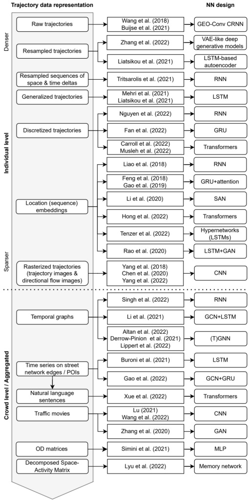
I’ve previously written about Movement data in GIS and the AI hype and today’s post is a follow-up in which I want to share with you a new review of the state of the art in deep learning from trajectory data.

Our review covers 8 use cases:

  1. Location classification
  2. Arrival time prediction
  3. Traffic flow / activity prediction
  4. Trajectory prediction
  5. Trajectory classification
  6. Next location prediction
  7. Anomaly detection
  8. Synthetic data generation

We particularly looked into the trajectory data preprocessing steps and the specific movement data representation used as input to train the neutral networks:

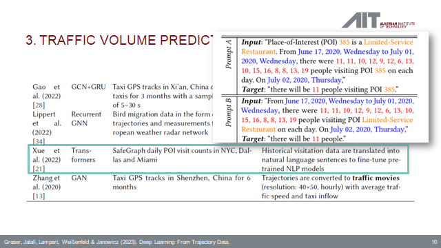
On a completely subjective note: the price for most surprising approach goes to natural language processing (NLP) Transfomers for traffic volume prediction.

The paper was presented at BMDA2023 and you can watch the full talk recording here:

References

Graser, A., Jalali, A., Lampert, J., Weißenfeld, A., & Janowicz, K. (2023). Deep Learning From Trajectory Data: a Review of Neural Networks and the Trajectory Data Representations to Train Them. Workshop on Big Mobility Data Analysis BMDA2023 in conjunction with EDBT/ICDT 2023.


This post is part of a series. Read more about movement data in GIS.

2.7.3 - Heroic Hedgehog

Changes

🐛 Bug Fixes

  • Significant improvement in Bluetooth connection reliability
  • Dark theme tweaks

  • <<
  • Page 12 of 141 ( 2809 posts )
  • >>

Back to Top

Sustaining Members