Get fieldwork smoothly and nimbly done despite the ice and snow outside. Collect accurate data with freehand digitizing and improved form widgets, use the data from your external GNSS receivers without any third-party apps and enjoy the pleasant usability of QField 1.8 Selma.

This year started off hi-speed for us. There’s been already a lot of coding, designing and teaching, and we’ve thrown ourselves into these things we love to do. And we published another QField release last week that I completely forgot to announce in this blog. But here it is. It’s QField 1.8, Selma. And it’s packed with cool features.

Let’s have a look.

Freehand drawing

This might be a feature that brings a lot of fun and professionalism to your work. The freehand digitizing mode allows the user to “draw” lines and polygons with the stylus pen. The mode is available for adding line/polygon features as well as for the ring tool of the geometry editor.

Together with the powerful options in the topological editing where you can snap to existing features and avoid overlaps, it’s very convenient to digitize complex shapes.

Zoom in and out

Speaking of fun. One day, a guy from the QGIS community asked us if we could implement the functionality to zoom in and zoom out like he is able to do with an app called Maps from a company named Google. I didn’t know what he meant, but he explained: Single finger double tap-and-hold zoom gesture (which allows you to zoom smoothly from anywhere on the screen). Wow! Didn’t know it before, but it’s super neat! So we made it available in QField as well.

If you are used to it, it’s quite easy. But for beginners it can be a bit difficult. So for people who are not that deft – and to keep the UX self-explanatory and simple – we also added two buttons + / – to zoom in and zoom out with just one finger. So now even a clumsy pirate with a hook instead of a hand can collect data with QField

Powerful Relation Reference Widget

Let’s be a little bit more serious and talk about how powerful the relation reference widget has become.

View and Edit selected feature

The intuitive eye icon next to the widget lets you open the form of the referenced parent feature to view and edit it.

Autocomplete mode

When auto-complete is enabled, you can easily perform a search in all available parent features.

With space-separated input, you can search for the beginning of multiple words in the display name of the parent features. So in this example searching for “Ma” will find the name “Mae” and “Marie” and using the second word “buck” it finds the Buckfast bees – so the entries containing both values will be listed on top.

Integration of external GNSS receivers

In case you wondered, why we did not release 1.8 Selma earlier? Because we wanted to have it feature loaded and rocket proof. And one of this cool feature is the integration of external GNSS receivers.

QField can receive and decode NMEA sentences received via Bluetooth from an external GNSS receiver (such as an EMLID Reach RS2) without the need for any third party app.

Search for paired Bluetooth devices in the device settings, connect to the external device and receive the GNSS information.

Select vertical grid shift files

In the QField settings, you can select a grid file on your mobile device by placing it in a directory named QField/proj in the main folder of the internal storage to increase the vertical location accuracy.

Postgres Config File

If you once started using PostgreSQL configuration files, you don’t want to live without them anymore. And when you use it on your PC, I’m sure you want to use it on your mobile device as well.

Define Postgresql services in a pg_service.conf file and use it on QField by placing it directly in a directory named QField in the main folder of the internal storage.

Add reload data button

The layer properties have been polished and in addition, you will find a button to reload the layer data. This is especially useful if you use WFS layers from which you need to get updates.

Register extra fonts

Also, you can add TTF and OTF font files into a directory named QField/fonts at the main folder of the internal storage to use the nice fonts you like.

How beautiful is that!

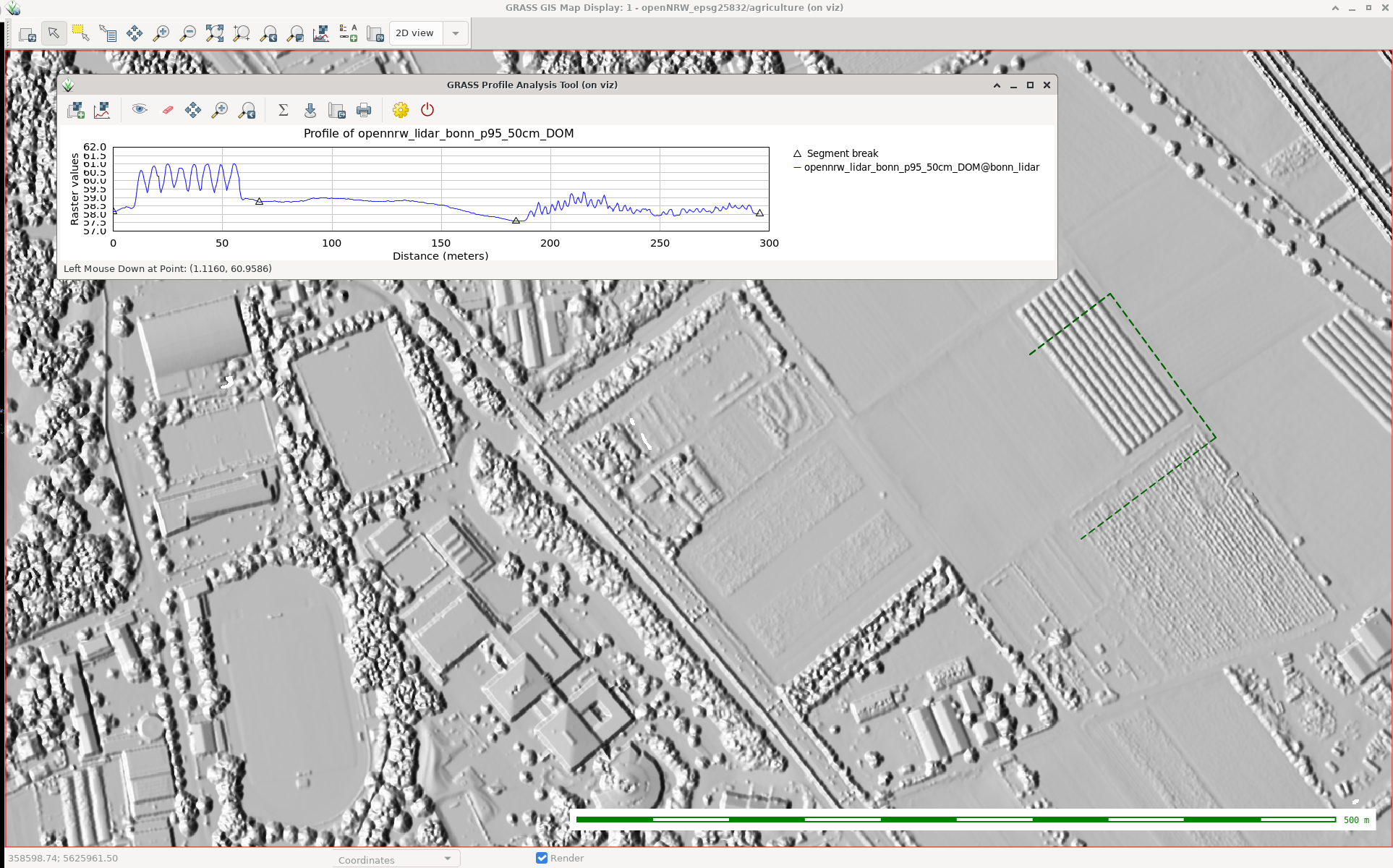
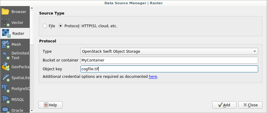
Support of new raster file formats

By the way: Many new raster file formats are supported – most notably COG. While not yet supported as remote format streamed directly from the web, it is also a high performance format if used locally

What about the cloud?

You might be one of these people eagerly waiting and always receiving the same message: Keep calm, it’s coming soon. Sorry for that. But when we do something, we do it right. And we prefer to have a stable solution than to publish half baked stuff. We are still highly busy coding, testing and promoting QFieldCloud. It’s announced for this spring / early summer.

Also, keep an eye on the @QFieldForQgis and @QFieldCloud twitter accounts to stay updated.

We our Beta Testers

The Beta Testers are our secret heroes. They report bugs and inconveniences before the normal users are bothered with them. Thanks to the Beta Testers QField is so stable. And at this point we would like to say: Thank you, test heroes!

And what do the beta testers get in return? Well, they can be the very first to try out the great new features. This is exciting and fun. So don’t hesitate. Join the beta.

In the Play Store you should find this section under the “QField for QGIS” app listing. Enjoy the feature frenzy and report the problems at qfield.org/issues

And if you wondered…

… why this release is called “Selma”. It’s of course because of the Mount Selma in Australia… And because it’s the name of my beloved cat. That’s her – Selma Eulenkopf – staring at me while I’m coding QField.

Data sourcing and preparation is one of the most time consuming tasks in many spatial analyses. Even though the Austrian data.gv.at platform already provides a central catalog, the individual datasets still vary considerably in their accessibility or readiness for use.

OGD.AT Lab is a new repository collecting Jupyter notebooks for working with Austrian Open Government Data and other auxiliary open data sources. The notebooks illustrate different use cases, including so far:

1. Accessing geodata from the city of Vienna WFS
2. Downloading environmental data (heat vulnerability and air quality)
3. Geocoding addresses and getting elevation information
4. Exploring urban movement data

Data processing and visualization are performed using Pandas, GeoPandas, and Holoviews. GeoPandas makes it straighforward to use data from WFS. Therefore, OGD.AT Lab can provide one universal gdf_from_wfs() function which takes the desired WFS layer as an argument and returns a GeoPandas.GeoDataFrame that is ready for analysis:

Launch this notebook in: https://mybinder.org/v2/gh/anitagraser/ogd-at-lab/v0.1?urlpath=lab/tree/notebooks/wien-ogd.ipynb

Many other datasets are provided as CSV files which need to be joined with spatial datasets to use them in spatial analysis. For example, the “Urban heat vulnerability index” dataset which needs to be joined to statistical areas.

Launch this notebook in Mybinder: https://mybinder.org/v2/gh/anitagraser/ogd-at-lab/v0.1?urlpath=lab/tree/notebooks/environment.ipynb

Another issue with many CSV files is that they use German number formatting, where commas are used as a decimal separater instead of dots:

Besides file access, there are also open services provided by other developers, for example, Manfred Egger developed an elevation service that provides elevation information for any point in Austria. In combination with geocoding services, such as Nominatim, this makes is possible to, for example, find the elevation for any address in Austria:

Launch this notebook in MyBinder: https://mybinder.org/v2/gh/anitagraser/ogd-at-lab/v0.1?urlpath=lab/tree/notebooks/elevation.ipynb

Last but not least, the first version of the mobility notebook showcases open travel time data provided by Uber Movement:

Launch this notebook in Mybinder: https://mybinder.org/v2/gh/anitagraser/ogd-at-lab/v0.1?urlpath=lab/tree/notebooks/mobility.ipynb

The utility functions for data access included in this repository will continue to grow as new data sources are included. Eventually, it may make sense to extract the data access function into a dedicated library, similar to geofi (Finland) or geobr (Brazil).

If you’re aware of any interesting open datasets or services that should be included in OGD.AT, feel free to reach out here or on Github through the issue tracker or by providing a pull request.

What’s new in a nutshell

As a follow-up to the previous GRASS GIS 7.8.4 we have published the new release GRASS GIS 7.8.5 with more than 80 improvements. This minor release offers new wxGUI fixes across the tree. Also the addon extension manager received various stability fixes. VRT raster map with tiled raster maps can now be properly exported and imported in the native GRASS GIS raster format.

The overview of new features in the 7.8 release series is available at new features in GRASS GIS 7.8. See also our detailed announcement with the full list of changes and bugs fixed at https://trac.osgeo.org/grass/wiki/Release/7.8.5-News.

Binaries/Installer download:

• winGRASS 7.8.5/standalone: 32bit standalone installer | 64bit standalone installer
• winGRASS 7.8.5/OSGeo4W: 32bit OSGeo4W installer | 64bit OSGeo4W installer
• Mac
• Linux
  • Debian
  • Fedora/Centos/EPEL
  • Ubuntu
  • … further binary packages for other Linux distributions will follow shortly, please check at software downloads

Source code download:

• https://grass.osgeo.org/grass78/source/
• https://grass.osgeo.org/grass78/source/grass-7.8.5.tar.gz
• To get the GRASS GIS 7.8.5 source code directly from GitHub, see here.

First time users may explore the first steps tutorial after installation.

About GRASS GIS

The Geographic Resources Analysis Support System (https://grass.osgeo.org/), commonly referred to as GRASS GIS, is an Open Source Geographic Information System providing powerful raster, vector and geospatial processing capabilities. It can be used either as a stand-alone application or as backend for other software packages such as QGIS and R geostatistics or in the cloud. It is distributed freely under the terms of the GNU General Public License (GPL). GRASS GIS is a founding member of the Open Source Geospatial Foundation (OSGeo).

The GRASS Development Team, Dec 2020

The post GRASS GIS 7.8.5 released appeared first on Markus Neteler Consulting.

In episode 86 of MapScaping podcast, Markus Neteler talks about the functionality offered (the topological vector engine, 2D and 3D raster analysis, image processing and available programming interfaces), and whom GRASS GIS is for.

Markus is the cofounder of mundialis, a Bonn based business. He is also the Chairman of the GRASS GIS Project Steering Committee.

Enjoy the podcast and the transcript!

The post MapScaping podcast: GRASS GIS probably doesn’t get the attention it deserves appeared first on Markus Neteler | Geospatial Analysis | Remote sensing | GRASS GIS.

Be ready for the cold weather with a smooth coordinate search, filters in the value relation widget, fancy new QML and HTML widgets, enhanced geometry editing functionalities and an expandable legend. Right when Autumn starts, QField 1.7 Rockies hits the stage.

As usual get it now on the play store or on github!

The days are getting shorter and the wind blows colder. It’s always good to be in a good company outside while getting your mapping work done. QField will be your reliable companion.

We know, QField 1.6 Qinling has only been out two months and with its amount of new features and stability improvements, it would have deserved a longer primetime. But we just couldn’t withhold you all the new great stuff we’ve been building lately.

So let’s welcome QField 1.7 Rockies. And yes, we mean THE Rockies, where QField is looking for plenty of new buddies.

Let’s have a look.

Merging features

Splitting of a feature has been possible for quite some time. Now the merging of features of multipolygon-layer is possible as well. Select them and merge them – easy like that. The first selected feature gets the new geometry and keeps its attributes.

Filters in the Value Relation Widget

The value relation widgets provide an easy selection of a related feature. Often it’s used for lookup tables but sometimes the related tables contain a lot of entries and the list of the possible values is long.

Using filters in the value relation drop-down can increase the efficiency in selecting the correct value. It can be configured by expressions in QGIS, so it’s possible to have the content of the drop down depend on the values entered previously in other fields.

In the screenshot above there is a Map Value Widget with “forest” and “meadow” as values. On selecting “forest”, only the trees appear in the Field “Plant Species”. On selecting “meadow” there would be listed flowers instead.

Go to coordinates in the Search

The search has not only been improved in its appearance, but it’s handling is much more comfortable with a button to clear the text and easy opening and closing.

Additionally, we added the possibility to jump to coordinates. Searching a place you know the coordinates of is now super simple. And this means that digitizing that precise geometry with known coordinates is finally possible.

QML and HTML Widget

You might remember when we introduced the QML widget in QGIS. Now it’s in QField as well. And it’s not alone. HTML widgets are supported too.

This provides a lot of possibilities to display information with texts, images and charts and it even allows you interaction.
Do you need help setting up complex forms? Don’t hesitate to get in touch with us!

Expandable legend icons

The legend items are now expandable and collapsible.

Wait a minute… Wasn’t this possible before? Yes. It was possible in earlier versions. But why it’s announced here as a new feature?

Because now it is built in a future proof manner thanks to all the people and organisations who care for QField and bought a support contract with the sustainability initiative or committed to a recurring sponsorship.

Some technical background: As you may be aware QField uses QGIS under the hood and QGIS uses Qt under the hood. Qt is currently used in version 5. Qt 5 is not that young any more and has a lot of functionality which is no longer supported by Qt. The old legend was based on the tree view, a deprecated module. Using it had some implications like the suboptimal support of HiDPI. Furthermore, these deprecated modules will disappear in the soon-to-come Qt 6.

As you can see, keeping QField at the quality we and you expect requires a lot of maintenance work. It is of utmost importance and only possible thanks to sponsoring since paying for fixing already existing features is less attractive for most people.

What will the future bring

In the last weeks, we have been highly busy on coding, testing and promoting QFieldCloud and we are very happy to be able to announce it very soon. So be prepared.

Also, keep an eye on the @QFieldForQgis and @QFieldCloud twitter accounts to stay updated.

Open Source

QField is an open source project. This means that whatever is produced is available free of charge. To anyone. Forever. This also means that everyone has the chance to contribute. You can write code, but you don’t need to. You can also help translating the app to your language or help out writing documentation or case studies or by sponsoring a new feature.

And now…

… enjoy QField 1.7 Rockies and have a nice autumn!

1. What’s new in a nutshell

As a follow-up to the previous GRASS GIS 7.8.3 we have published the new release GRASS GIS 7.8.4 with more than 170 improvements. This minor release again focuses on wxGUI fixes, especially in the animation export, the layer management, 3D visualization and the data catalogue. Many display modules received fixes as well, and the vector digitizer now works as expected.

The overview of new features in the 7.8 release series is available at new features in GRASS GIS 7.8. See also our detailed announcement with the full list of changes and bugs fixed at https://trac.osgeo.org/grass/wiki/Release/7.8.4-News.

Binaries/Installer download:

• winGRASS 7.8.4/standalone: 32bit standalone installer | 64bit standalone installer
• winGRASS 7.8.4/OSGeo4W: 32bit OSGeo4W installer | 64bit OSGeo4W installer
• Mac
• Linux
  • Debian
  • Fedora/Centos/EPEL
  • Ubuntu
  • … further binary packages for other Linux distributions will follow shortly, please check at software downloads

Source code download:

• https://grass.osgeo.org/grass78/source/
• https://grass.osgeo.org/grass78/source/grass-7.8.4.tar.gz
• To get the GRASS GIS 7.8.4 source code directly from GitHub, see here.

First time users may explore the first steps tutorial after installation.

About GRASS GIS

The Geographic Resources Analysis Support System (https://grass.osgeo.org/), commonly referred to as GRASS GIS, is an Open Source Geographic Information System providing powerful raster, vector and geospatial processing capabilities. It can be used either as a stand-alone application or as backend for other software packages such as QGIS and R geostatistics or in the cloud. It is distributed freely under the terms of the GNU General Public License (GPL). GRASS GIS is a founding member of the Open Source Geospatial Foundation (OSGeo).

The GRASS Development Team, Oct 2020

The post GRASS GIS 7.8.4 released appeared first on GFOSS Blog | GRASS GIS and OSGeo News.

We have recently been working for the French Space Agency ( CNES ) who needed to store and visualize satellite rasters in a cloud platform. They want to access the image raw data, with no transformation, in order to fullfill deep analysis like instrument calibration. Using classic cartographic server standard like WMS or TMS is not an option because those services transform datasets in already rendered tiles.

We chose to use a quite recent format managed by GDAL, the COG (Cloud Optimize Geotiff) and target OVH cloud platform for it provides OpenStack, a open source cloud computing platform.

How it works

A COG file is a GEOTiff file which inner structure is tiled, meaning that the whole picture is divided in fixed size tile (256 x 256 pixels for instance) so you can efficiently retrieve parts of the raster. In addition to the HTTP/1.1 standard feature range request, it is possible to get specific tiles of an image through the network without downloading the entire raster.

We used a service provided by OpenStack, called Object Storage to serve the COG imagery. Object storage allows to store and retrieve file as objects using HTTP GET/POST requests.

Why not WCS ?

Web Coverage Service standard could have been an option. A WCS server can serve raw data according to a given geographic extent. It’s completely possible to deploy a container or a VPS (Virtual Private Server) running a WCS Server in a cloud plateform. The main advantages of the COG solution over WCS Server is that you don’t have to deal with the burden of deploying a server, like giving it ressources, configuring load balancing, handle updates, etc…

The beauty of COG solution is its simplicity. It is only HTTP requests, and everything else (rendering for instance) is done on the client side.

Step by step

Here are the different steps you’d have to go through if you’re willing to navigate in a big raster image directly from the cloud.

First, let’s generate a COG file

gdal_translate inputfile.tif cogfile.tif -co TILED=YES -co COPY_SRC_OVERVIEWS=YES -co COMPRESS=DEFLATE

Install your openstack-client, it can be achieved easily with Python pip install command line

$ pip install python-openstackclient

Next, configure your openstack client in order to generate an athentification token. To do so you need to download your project specific openrc file to setup your environment)

$ source myproject-openrc.sh
Please enter your OpenStack Password for project myproject as user myuser:
**********
$ openstack token issue                                 
+------------+-----------------------------------------------------------------------------------------------------------------------------------------------------------------------------------------+
| Field      | Value                                                                                                                                                                                   |
+------------+-----------------------------------------------------------------------------------------------------------------------------------------------------------------------------------------+
| expires    | 2020-07-21T08:15:12+0000                                                                                                                                                                |
| id         | xxxx_my_token_xxxx
| project_id | 97e2e750f1904b41b76f80a50dabde0a                                                                                                                                                        |
| user_id    | 18f7ccaf1a2d4344a4e35f0d84eb065e                                                                                                                                                        |
+------------+-----------------------------------------------------------------------------------------------------------------------------------------------------------------------------------------+

You are now good to push you COG file to the cloud instance

openstack object create MyContainer cogfile.tif --name cogfile.tif

Before starting QGIS, 2 environment variables need to be set.  (replace xxxx_my_token_xxxx with the token you’d just come to generate)

$ export SWIFT_AUTH_TOKEN=xxxx_my_token_xxxx
$ export SWIFT_STORAGE_URL=https://storage.sbg.cloud.ovh.net/v1/AUTH_$OS_PROJECT_ID

It can also be done directly from the QGIS Python console by setting those variable using the os.environ.

Finally, add a cloud raster data source in in QGIS

You can now navigating into your image directly reading it from the cloud

© CNES 2018, Distribution Airbus DS

Performances

While panning in the map, QGIS will download only few tiles from the image in order to cover the view extent. The display latency that you could see in the video depends essentially on:

• The number of band of your image
• The pixel size
• Your internet connection (mine, the one use for the video, is not an awesome one)

Note that the white flickering that you could see when you move in the map and the raster is refreshed should be removed in next version of QGIS according to this QEP.

What’s next ?

Thanks so much to the GDAL and QGIS contributors for adding such a nice feature ! It brings lots of possibilities for organizations that have to deal with great number of big raster and just want to explore part of it.

We are already thinking about further improvments (ease authentification, better integration with processing…), so if you’re willing to fund them or just want to know more about QGIS, feel free to contact us at [email protected]. And please have a look at our support offering for QGIS.

On Thursday, I was awarded the 2020 Sol Katz award for Free and Open Source Software for Geospatial. I feel very honored to have been selected for this award and I’d like to take this opportunity to share a few words of thanks:

As people working in open source projects, we are constantly reminded that we are all standing on the shoulders of giants. However, particularly this year, we also see just how important small personal connections are. For me, my involvement with open source communities really took off when I joined the QGIS hackfest in Vienna in 2009 and I felt that my participation was really appreciated and welcome. I couldn’t imagine being without these connections anymore.

Thank you to the whole QGIS community, particularly my fellow PSC members both current and former: Tim, Andreas, Jürgen, Richard, Paolo, Otto, Marco Hugentobler, Alessandro, our new chair Marco Bernasocchi, and of course QGIS founder Gary Sherman for starting this awesome project and for still being around and actively promoting geospatial open source by publishing so many great books covering multiple different OSGeo projects.

I’d also like to thank my partner and my family for being incredibly understanding whenever I’m spend my time geeking out over a new programming project, data analysis, forum question, or conference talk.

Thank you also to my friends, colleagues and fellow members of the larger OSGeo community for sharing ideas, providing valuable feedback, and spreading the word about all the great work that’s going on all around us.

I’m constantly amazed by all the innovation happening to nourish and grow our community. And I’m looking forward to continue being a part of these efforts.

Thank you!

Rendering large sets of trajectory lines gets messy fast. Different aggregation approaches have been developed to address this issue. However, most approaches, such as mobility graphs or generalized flow maps, cannot handle large input datasets. Building on M³ prototypes, the following approach can be used in distributed computing environments to extracts flows from large datasets. 

This is part 3 of “Exploring massive movement datasets”.

This flow extraction is based on a two-step process, conceptually similar to Andrienko flow maps: first, we extract M³ prototypes from the movement data. In the second step, we determine flows between these prototypes, including information about: distribution of travel speeds and number of observed transitions. The resulting flows can be visualized, for example, to explore the popularity of different paths of movement:

After the prototypes have been computed, the flow algorithm computes transitions between pairs of prototypes. An object moving from prototype A to prototype B triggers an update of the corresponding flow. To allow for distributed processing, each node in the distributed computing environment needs a copy of the previously computed prototypes. Additionally, the raw movement data records need to be converted into trajectories. Afterwards, each trajectory is processed independently, going through its records in chronological order:

1. Find the best matching prototype for the current record
2. Ensure that the distance to the match is below the distance threshold and that the matched prototype is different from the previous prototype
3. Get or create the flow between the two prototypes
4. Ensure that the prototype and flow directions are a good match for the current record’s direction
5. Update the flow properties: travel speed and number of transitions, as well as the previous prototype reference

This approach scales to large datasets since only the prototypes, the (intermediate) flow results, and the trajectory currently being worked on have to be kept in memory for each iteration. However, this algorithm does not allow for continuous updates. Flows would have to be recomputed (at least locally) whenever prototypes changed. Therefore, the algorithm does not support exploration of continuous data streams. However, it can be used to explore large historical datasets:

Flow example: passenger vessel speed patterns showing mean flow speeds (line color: darker colors equal higher speeds) and speed variation (line width)

If you want to dive deeper, here’s the full paper:

[1] Graser, A., Widhalm, P., & Dragaschnig, M. (2020). Extracting Patterns from Large Movement Datasets. GI_Forum – Journal of Geographic Information Science, 1-2020, 153-163. doi:10.1553/giscience2020_01_s153.

This post is part of a series. Read more about movement data in GIS.

Editing multiple features at the same time, support for stylus pens, dynamic configuration of image names and much more.
QField 1.6 Qinling 秦岭 comes packed with awesome new features and an improved user experience.

We have been very busy over the last few months working on a new and shiny QField release. We have added many new features that increase efficiency on the field or allow for new workflows. In parallel, we have also been working on ironing out a series of issues and improving the overall user experience to make the app as pleasurable to use as possible. The result is QField 1.6 which has been published now.

Enough of the highlevel talking, let’s see what has been done.

Multi editing

Do you recall Geography lesson 101, Toblers first law? Everything is related to everything else. But near things are more related than distant things.

Very often there are similar objects nearby which share a property, tree species tend to group, human created objects like street light types or street paint markings tend to be of the same type at the same location.

With QField 1.6 it is now much easier to select a couple of features and change an attribute with very few taps. Identify a feature, long press an identify results, select more features and click the edit attributes button.

Stylus support

Sometimes it is just too cold to be working with fingers (although of course you can get capacitive gloves too). Or you just prefer to be working with a pen. QField 1.6 comes with support for stylus pens. If your device ships with one, give it a try.

Lock geometries

For some scenarios, especially in asset management, you only need to change attributes of existing objects and never add new features, delete features or change geometries. This can be configured through QFieldSync and set in the layer properties.

Image name configuration

Did you ever want to have the file names of your pictures to match the feature id, the layer name or any free text? The expression based configuration in QFieldSync offers now complete freedom in naming your images.

Legend and UX and legacy code

Didn’t expect to read UX and legacy code in one single title?

QML is the technology on which the QField user interface is built. QML ships a lot of user interface elements in a library called “Quick Controls”. A long time ago already it received an update from version 1 to version 2. Up to recently we still have been using some elements from version 1, which had an effect on high resolution displays not being able to properly display everything. To workaround that we introduced a lot of band aids, to improve the situation. We are very happy, that by migrating the legend and few other remaining elements to Quick Controls 2 in version 1.6, we have been able to completely drop this code.

Topological editing

QGIS can detect shared boundary by the features, so you only have to move a common vertex once, and QGIS will take care of updating the neighboring ones. So does his little college QField since this release.

Fast editing mode

For the real adventurers who know what they are doing this release brings the fast editing mode. In this mode, the features will automatically be stored on every change. The user interface is lighter and it combines perfectly with the topological editing.

Unter the hood

We have brought the whole technology stack up to speed with modern requirements. Proj and GDAL have been updated to recent versions. This helped to mitigate a couple of issues with coordinate transformations that were completely misplaced. It also paves the path for a future with datum corrections and always more important high precision measurements.

Known Issues

Unfortunately, we are experiencing a crash on startup with 32 bit devices. These devices are not that common any more, but if you have a device that is already a couple of years old it’s very well possible that it comes with a 32 bit cpu builtin. Despite the team’s hard efforts to isolate the reason, we were not able to find out what it was yet. Because of this we will not be able to update to 1.6 for these devices at the moment. We still hope that we will find a solution for this but don’t know yet when this will be.

We have updated proj to version 6. This brings plenty of bug fixes with coordinate handling. Among other things it adds support for using datum grids (gsb files) for very precise transformations, it is not yet possible to install those on the device. You will get an information message in the about dialog if your project happens to fall into this category. In this case, as a workaround switch the CRS of the project to a CRS with a known conversion that works without grid files.

What will the future bring

You guessed it already, we are not tired and have plenty of things stacked for the future. Prepare for more exciting updates for attribute forms and also for QFieldCloud which is right now being tested in our R&D labs.

Also keep an eye on the @QFieldForQgis Twitter account to stay updated.

Open Source

QField is an open source project. This means that whatever is produced is available free of charge. To anyone. Forever. This also means that everyone has the chance to contribute. You can write code, but you don’t need to. You can also help translating the app to your language or help out writing documentation or case studies or by sponsoring a new feature.

Thanks to sponsors

Various organisations have helped to make this new release become a reality. Without the support of people in organisations who believe in the future of QField and open source tool for geospatial in general. The whole team behind QField would like to thank you with a big applause!

To explore travel patterns like origin-destination relationships, we need to identify individual trips with their start/end locations and trajectories between them. Extracting these trajectories from large datasets can be challenging, particularly if the records of individual moving objects don’t fit into memory anymore and if the spatial and temporal extent varies widely (as is the case with ship data, where individual vessel journeys can take weeks while crossing multiple oceans). 

This is part 2 of “Exploring massive movement datasets”.

Roughly speaking, trip trajectories can be generated by first connecting consecutive records into continuous tracks and then splitting them at stops. This general approach applies to many different movement datasets. However, the processing details (e.g. stop detection parameters) and preprocessing steps (e.g. removing outliers) vary depending on input dataset characteristics.

For example, in our paper [1], we extracted vessel journeys from AIS data which meant that we also had to account for observation gaps when ships leave the observable (usually coastal) areas. In the accompanying 10-minute talk, I went through a 4-step trajectory exploration workflow for assessing our dataset’s potential for travel time prediction:

Click to watch the recorded talk

Like the M³ prototype computation presented in part 1, our trajectory aggregation approach is implemented in Spark. The challenges are both the massive amounts of trajectory data and the fact that operations only produce correct results if applied to a complete and chronologically sorted set of location records.This is challenging because Spark core libraries (version 2.4.5 at the time) are mostly geared towards dealing with unsorted data. This means that, when using high-level Spark core functionality incorrectly, an aggregator needs to collect and sort the entire track in the main memory of a single processing node. Consequently, when dealing with large datasets, out-of-memory errors are frequently encountered.

To solve this challenge, our implementation is based on the Secondary Sort pattern and on Spark’s aggregator concept. Secondary Sort takes care to first group records by a key (e.g. the moving object id), and only in the second step, when iterating over the records of a group, the records are sorted (e.g. chronologically). The resulting iterator can be used by an aggregator that implements the logic required to build trajectories based on gaps and stops detected in the dataset.

If you want to dive deeper, here’s the full paper:

[1] Graser, A., Dragaschnig, M., Widhalm, P., Koller, H., & Brändle, N. (2020). Exploratory Trajectory Analysis for Massive Historical AIS Datasets. In: 21st IEEE International Conference on Mobile Data Management (MDM) 2020. doi:10.1109/MDM48529.2020.00059

This post is part of a series. Read more about movement data in GIS.

Exploring large movement datasets is hard because visualizations of movement data quickly get cluttered and hard to interpret. Therefore, we need to aggregate the data. Density maps are commonly used since they are readily available and quick to compute but they provide only very limited insight. In contrast, meaningful aggregations that can help discover patterns are computationally expensive and therefore slow to generate.

This post serves as a starting point for a series of new approaches to exploring massive movement data. This series will summarize parts of my PhD research and – for those of you who are interested in more details – there will be links to the relevant papers.

Starting with the raw location records, we use different forms of aggregation to learn more about what information a movement dataset contains:

1. Summarizing movement using prototypes by aggregating raw location records using our flexible M³ Massive Movement Model [1]
2. Generating trajectories by connecting consecutive records into continuous tracks and splitting them into meaningful trajectories [2]
3. Extracting flows by summarizing trajectory-based transitions between prototypes [3]

Besides clever aggregation approaches, massive movement datasets also require appropriate computing resources. To ensure that we can efficiently explore large datasets, we have implemented the above mentioned aggregation steps in Spark. This enables us to run the computations on general purpose computing clusters that can be scaled according to the dataset size.

In the next post, we’ll look at how to summarize movement using M³ prototypes. So stay tuned!

But if you don’t want to wait, these are the original papers:

[1] Graser. A., Widhalm, P., & Dragaschnig, M. (2020). The M³ massive movement model: a distributed incrementally updatable solution for big movement data exploration. International Journal of Geographical Information Science. doi:10.1080/13658816.2020.1776293.
[2] Graser, A., Dragaschnig, M., Widhalm, P., Koller, H., & Brändle, N. (2020). Exploratory Trajectory Analysis for Massive Historical AIS Datasets. In: 21st IEEE International Conference on Mobile Data Management (MDM) 2020. doi:10.1109/MDM48529.2020.00059
[3] Graser, A., Widhalm, P., & Dragaschnig, M. (2020). Extracting Patterns from Large Movement Datasets. GI_Forum – Journal of Geographic Information Science, 1-2020, 153-163. doi:10.1553/giscience2020_01_s153.

This post is part of a series. Read more about movement data in GIS.

Podcasts have become huge. I’m an avid listener of podcasts myself. I particularly enjoy formats that take the time to talk about unconventional topics in detail.

My first podcast experience was on the QGIS podcast hosted by Tim Sutton in 2014. Unfortunately, it seems like the podcast episodes are not online anymore.

Recently, I had the pleasure to join the MapScaping Podcast by Daniel O’Donohue to talk about Python for Geospatial: 

Other guests Daniel has already interviewed include:

• Kurt Menke talking first about QGIS and in a second episode on QField and Input (data collection apps based on QGIS) and
• Paul Ramsey on Vector Tiles from PostGIS

Another geospatial podcast I really enjoy is The Mappyist Hour by Silas and Todd. Unfortunately, it’s a bit silent there now but it’s definitely worth to listen into their episode archive. One of my favorites is Episode 9 where Linda Stevens (Hecht) discusses her career at ESRI, the future of GIS, and the role of Open Source Spatial in that future:

If you listen to and want to recommend other spatial podcasts, please share them in the comments!

This is a guest post by Bommakanti Krishna Chaitanya @chaitan94

Introduction

This post introduces mobilitydb-sqlalchemy, a tool I’m developing to make it easier for developers to use movement data in web applications. Many web developers use Object Relational Mappers such as SQLAlchemy to read/write Python objects from/to a database.

Mobilitydb-sqlalchemy integrates the moving objects database MobilityDB into SQLAlchemy and Flask. This is an important step towards dealing with trajectory data using appropriate spatiotemporal data structures rather than plain spatial points or polylines.

To make it even better, mobilitydb-sqlalchemy also supports MovingPandas. This makes it possible to write MovingPandas trajectory objects directly to MobilityDB.

For this post, I have made a demo application which you can find live at https://mobilitydb-sqlalchemy-demo.adonmo.com/. The code for this demo app is open source and available on GitHub. Feel free to explore both the demo app and code!

In the following sections, I will explain the most important parts of this demo app, to show how to use mobilitydb-sqlalchemy in your own webapp. If you want to reproduce this demo, you can clone the demo repository and do a “docker-compose up –build” as it automatically sets up this docker image for you along with running the backend and frontend. Just follow the instructions in README.md for more details.

Declaring your models

For the demo, we used a very simple table – with just two columns – an id and a tgeompoint column for the trip data. Using mobilitydb-sqlalchemy this is as simple as defining any regular table:

from flask_sqlalchemy import SQLAlchemy
from mobilitydb_sqlalchemy import TGeomPoint

db = SQLAlchemy()

class Trips(db.Model):
   __tablename__ = "trips"
   trip_id = db.Column(db.Integer, primary_key=True)
   trip = db.Column(TGeomPoint)

Note: The library also allows you to use the Trajectory class from MovingPandas as well. More about this is explained later in this tutorial.

Populating data

When adding data to the table, mobilitydb-sqlalchemy expects data in the tgeompoint column to be a time indexed pandas dataframe, with two columns – one for the spatial data  called “geometry” with Shapely Point objects and one for the temporal data “t” as regular python datetime objects.

from datetime import datetime
from shapely.geometry import Point

# Prepare and insert the data
# Typically it won’t be hardcoded like this, but it might be coming from 
# other data sources like a different database or maybe csv files
df = pd.DataFrame(
   [
       {"geometry": Point(0, 0), "t": datetime(2012, 1, 1, 8, 0, 0),},
       {"geometry": Point(2, 0), "t": datetime(2012, 1, 1, 8, 10, 0),},
       {"geometry": Point(2, -1.9), "t": datetime(2012, 1, 1, 8, 15, 0),},
   ]
).set_index("t")

trip = Trips(trip_id=1, trip=df)
db.session.add(trip)
db.session.commit()

Writing queries

In the demo, you see two modes. Both modes were designed specifically to explain how functions defined within MobilityDB can be leveraged by our webapp.

1. All trips mode – In this mode, we extract all trip data, along with distance travelled within each trip, and the average speed in that trip, both computed by MobilityDB itself using the ‘length’, ‘speed’ and ‘twAvg’ functions. This example also shows that MobilityDB functions can be chained to form more complicated queries.

trips = db.session.query(
   Trips.trip_id,
   Trips.trip,
   func.length(Trips.trip),
   func.twAvg(func.speed(Trips.trip))
).all()

2. Spatial query mode – In this mode, we extract only selective trip data, filtered by a user-selected region of interest. We then make a query to MobilityDB to extract only the trips which pass through the specified region. We use MobilityDB’s ‘intersects’ function to achieve this filtering at the database level itself.

trips = db.session.query(
   Trips.trip_id,
   Trips.trip,
   func.length(Trips.trip),
   func.twAvg(func.speed(Trips.trip))
).filter(
   func.intersects(Point(lat, lng).buffer(0.01).wkb, Trips.trip),
).all()

Using MovingPandas Trajectory objects

Mobilitydb-sqlalchemy also provides first-class support for MovingPandas Trajectory objects, which can be installed as an optional dependency of this library. Using this Trajectory class instead of plain DataFrames allows us to make use of much richer functionality over trajectory data like analysis speed, interpolation, splitting and simplification of trajectory points, calculating bounding boxes, etc. To make use of this feature, you have set the use_movingpandas flag to True while declaring your model, as shown in the below code snippet.

class TripsWithMovingPandas(db.Model):
   __tablename__ = "trips"
   trip_id = db.Column(db.Integer, primary_key=True)
   trip = db.Column(TGeomPoint(use_movingpandas=True))

Now when you query over this table, you automatically get the data parsed into Trajectory objects without having to do anything else. This also works during insertion of data – you can directly assign your movingpandas Trajectory objects to the trip column. In the below code snippet we show how inserting and querying works with movingpandas mode.

from datetime import datetime
from shapely.geometry import Point

# Prepare and insert the data
# Typically it won’t be hardcoded like this, but it might be coming from 
# other data sources like a different database or maybe csv files
df = pd.DataFrame(
   [
       {"geometry": Point(0, 0), "t": datetime(2012, 1, 1, 8, 0, 0),},
       {"geometry": Point(2, 0), "t": datetime(2012, 1, 1, 8, 10, 0),},
       {"geometry": Point(2, -1.9), "t": datetime(2012, 1, 1, 8, 15, 0),},
   ]
).set_index("t")

geo_df = GeoDataFrame(df)
traj = mpd.Trajectory(geo_df, 1)

trip = Trips(trip_id=1, trip=traj)
db.session.add(trip)
db.session.commit()

# Querying over this table would automatically map the resulting tgeompoint 
# column to movingpandas’ Trajectory class
result = db.session.query(TripsWithMovingPandas).filter(
   TripsWithMovingPandas.trip_id == 1
).first()

print(result.trip.__class__)
# <class 'movingpandas.trajectory.Trajectory'>

Bonus: trajectory data serialization

Along with mobilitydb-sqlalchemy, recently I have also released trajectory data serialization/compression libraries based on Google’s Encoded Polyline Format Algorithm, for python and javascript called trajectory and trajectory.js respectively. These libraries let you send trajectory data in a compressed format, resulting in smaller payloads if sending your data through human-readable serialization formats like JSON. In some of the internal APIs we use at Adonmo, we have seen this reduce our response sizes by more than half (>50%) sometimes upto 90%.

Want to learn more about mobilitydb-sqlalchemy? Check out the quick start & documentation.

This post is part of a series. Read more about movement data in GIS.

You are using QGIS and look for support services to improve your experience and solve problems ? Oslandia is here to help you with our full QGIS editor service range ! Discover our team members below.

You will probably interact first with our pre-sales engineer Bertrand Parpoil. He leads Geographical Information System projects for 15 years for large corporations, public administrations or hi-tech SME. Bertrand will listen to your needs and explore your use cases, to offer you the best set of services.

Régis Haubourg also takes part in the first steps of projects to analyze your usages and improve them. GIS Expert, he knows QGIS by heart and will make the most of its capabilities. As QGIS Community Manager at Oslandia, he is very active in the QGIS community of developers and contributors. He is president of the Francophone OSGeo local chapter ( OSGeo-fr ), QGIS voting member, organizes the French QGIS day conference in Montpellier, and participates to QGIS community meetings. Before joining Oslandia, he led the migration to QGIS and PostGIS at the Adour-Garonne Water Agency, and now guides our clients with their GIS migrations to OpenSource solutions. Régis is also a great asset when working on water, hydrology and other specific thematic subjects.

Loïc Bartoletti develops QGIS, specializing in features corresponding to his fields of interests : network management, topography, urbanism, architecture… We find him contributing to advanced vector editing in QGIS, writing Python plugins, namely for DICT management. Pushing CAD and migrations from CAD tools to GIS and QGIS is one of his major goals. He will develop your custom applications, combining technical expertise and functional competences. When bored, Loïc packages software on FreeBSD.

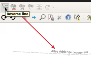
Vincent Mora is senior developer in Python and C++, as well as PostGIS expert. He has a strong experience in numerical simulation. He likes coupling GIS (PostGIS, QGIS) with 3D numerical computing for risk management or production optimization. Vincent is an official QGIS committer and can directly integrate your needs into the core of the software. He is also GDAL committer and optimizes low-level layers of your applications. Among numerous activities, Vincent serves as lead developer of the development team for Hydra Software, a tool dedicated to unified hydraulics and hydrology modelling and simulation based on QGIS.

Hugo Mercier is an officiel QGIS committer too for several years. He regularly talks in international conferences on PostGIS, QGIS and other OpenSource GIS softwares. He will implement your needs with new QGIS features, develop innovative plugins ( like QGeoloGIS ) and design and build your new custom applications, solving all kind of technological challenges.

Paul Blottière completes our QGIS committers : very active on core development, Paul has refactored the QGIS server component to bring it to an industry-grade quality level. He also designed and implemented the infrastructure allowing to guarantee QGIS server performances. He dedicated himself to QGIS server OGC certification, especially for WMS (1.3). Thanks to this work QGIS is now a reference OGC implementation.

Julien Cabièces recently joined Oslandia, and quickly dived into QGIS : he contributes to the core of this Desktop GIS, on the server component, as well as applications linked to numerical simulation. Coming from a satellite imagery company with industrial applications, he uses his flexibility to answer all your needs. He brings quality and professionalism to your projects, minimizing risks for large production deployments.

You may also meet Vincent Picavet. Oslandia’s founder is a QGIS.org voting member, and is involved in the project’s evolution and the organization of the community.

Aside from these core contributors, all other Oslandia members also master QGIS integrate this tool into their day-to-day projects.

Bertrand, Régis, Loïc, Vincent (x2), Hugo, Paul et Julien are in tune with you and will be happy to work together for your migrations, application development, and all your desires to contribute to the QGIS ecosystem. Do not hesitate to contact us !

A few months ago, we proposed to the QGIS grant program to make improvements to the snap cache in QGIS. The community vote selected our project which was funded by QGIS.org. Developments are now mostly finished.

In short, snapping is crucial for editing geospatial features. It is the only way to ensuring they are topologically related, ie, connected vertices have exactly the same coordinates even if manual digitizing on screen is imprecise by nature.  Snapping correctly supposes QGIS have in memory an indexed cache of the geometries to snap to. And maintainting this cache when data is modified, sometimes by another user or database logic, can be a real challenge. This it exactly what this work adresses.

The proposal was divided into two different tasks:

• Manage circular dependencies
• Relax the snap cache index build

Manage cicular data dependencies

Data dependencies

Data dependency is an existing feature that allows you to configure QGIS to reload layers (and their snapping cache) when a layer is modified.

It is useful when you store your data in a database and you set up triggers to maintain consistency between the different tables of your data model.

For instance, say you have topological informations containing lines and nodes. Nodes are part of lines and lines go through nodes. Then, you move a node in QGIS, and save your modifications to the database. In order to keep the data consistent, a trigger updates the geometry of the line going through the modified node.

Node 2 is modified, Line 1 is updated accordingly

QGIS, as a database client, has no information that the line layer currently displayed in the canvas needs to be refreshed after the trigger. Although the map canvas will be up to date, because QGIS fetches data for display without any caching system, the snapping cache is not and you’ll end up with ghost snapping highlights issues.

Snapping highlights (light red) differ from real line (orange)

Defining a dependency between nodes and lines layers tells QGIS that it has to refresh the line layer when a node is modified.

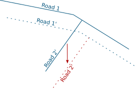
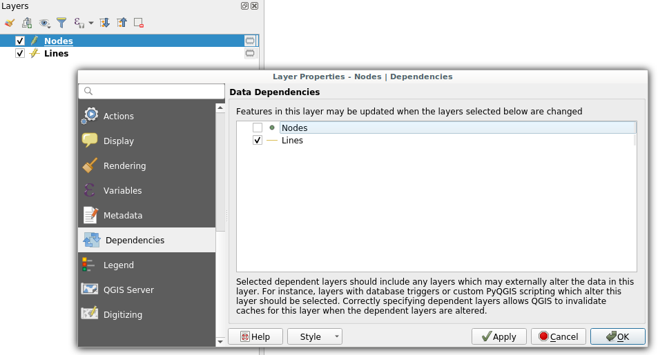Dependencies configuration: Lines layer will be refreshed whenever Nodes layer is modified

It also have to work the other way, modifying a line should update the nodes to ensure they still are on the line.

Circular data dependencies

So here we are, lines depend on nodes which depend on lines which depend on nodes which…

That’s what circular dependencies is about. This specific behavior was previously forbidden and needed a special way to deal with it. Thanks to this recent development, it is now possible.

It’s also possible to add the layer itself as one of its own dependencies. It helps dealing with specific cases where one feature modification could lead to a modification of another feature in the same layer (to keep consistency on road networks for instance).

Road 2 is modified, Road 1 is updated accordingly

This feature is available in the next QGIS LTR version 3.10.

Relax the snapping cache index build

If you work in QGIS with huge projects displaying a lot of vector data, and you enable snapping while editing these data, you probably already met this dialog:

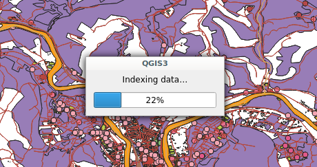Snap indexing dialog

This dialog informs you that data are currently being indexed so you can snap on them while you will edit feature geometry. And for big projects, this dialog can last for a really long time. Let’s work on speeding it up!

What’s a snap index?

Let’s say you want to move a line and snap it onto another one. While you drag your line with the mouse, QGIS will look for an existing geometry beneath the mouse cursor (with a certain pixel tolerance) every time you move your mouse. Without spatial index, QGIS will have to go through every geometry in your layer to check if the given geometry is beneath the cursor position. This would be very ineffective.

In order to prevent this, QGIS keeps an index where vector data are stored in a way that it can quickly find out what geometry is beneath the mouse cursor. The building of this data structure takes time and that is what the progress dialog is about.

Firstly: Parallelize snap index build

If you want to be able to snap on all layers in your project, then QGIS will have to build one snap index for each layer. This operation was made sequentially meaning that if you have for instance 20 layers and the index building last approximatively 3 seconds for each, then the whole index building will last 1 minute. We made modifications to QGIS so that index building could be done in parallel. As a result, the total index building time could theoretically be 3 seconds!

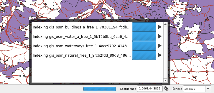4 layers snap index being built in parallel

However, parallel operations are limited by the number of CPU cores of your machine, meaning that if you have 4 cores (core i7 for instance) then the total time will be up to 4 times faster than when the building is sequential (and last 15 seconds in our example).

Secondly: relax the snap build

For big projects, parallelizing index building is not enough and still takes too much time. Futhermore, to reduce snap index building, an existing optimisation was to build the spatial index for a specific area of interest (determined according to the displayed area and layer size). As a consequence, when you’ve done waiting for an index currently building and you move the map or zoom in/out, you could possibly trigger another snap index building and wait again.

So, the idea was to avoid waiting at all. Snap index is now built whenever it needs to (when you first enable snapping, when you move or zoom) but the user doesn’t have to wait for the build to be over and can continue what it was doing (creating feature, moving…). Snapping highlights will be missing when the index is currently being built and will appear gradually as soon as they finished. That’s what we call the relaxing mode.

No waiting dialog, snapping highlights appears as soon as snap index is ready

This feature has been merged into current QGIS master and will be present in future QGIS 3.12 release. We keep working on this feature in order to make it more stable and efficient.

What’s next

We’ll continue to improve this feature in the coming days, if you have the chance to test it and encounter issues please let us know on the QGIS tracker. If you think about a missing feature or just want to know more about QGIS, feel free to contact us at [email protected]. And please have a look at our support offering for QGIS.

Many thanks to QGIS grant program for funding these new features. Thanks also to all the people involved in reviewing the code and helping to better understand the existing mechanism.

GRASS GIS 7.8.2 released with updated PROJ 6 and GDAL 3 support

What’s new in a nutshell

As a follow-up to the recent GRASS GIS 7.8.1 we have pusblished the new stable release GRASS GIS 7.8.2.
Besides other improvements, the release contains important PROJ 4/5/6 related datum handling fixes, wxGUI fixes and a fix for the vector import from PostGIS databases.

An overview of the new features in the 7.8 release series is available at new features in GRASS GIS 7.8.

Binaries/Installer download:

• winGRASS 7.8.2: 32bit standalone installer | 64bit standalone installer
• winGRASS 7.8.2 OSGeo4W: 32bit OSGeo4W installer | 64bit OSGeo4W installer
• Debian (forthcoming)
• Fedora and EPEL7 (CentOS7, RHEL7, … – included in Fedora 31+)
• Linux Mint: see Ubuntu
• Ubuntu (ubuntugis-unstable)
• … further binary packages for other Linux distributions will follow shortly, please check at software downloads.
  

Source code download:

• https://grass.osgeo.org/grass78/source/
• https://grass.osgeo.org/grass78/source/grass-7.8.2.tar.gz
• To get the GRASS GIS 7.8.2 source code directly from GitHub, see here.

See also our detailed announcement:

• https://trac.osgeo.org/grass/wiki/Release/7.8.2-News
• https://trac.osgeo.org/grass/wiki/Grass7/NewFeatures78 (overview of new 7.8 stable release series)
• https://grass.osgeo.org/grass7/manuals/addons/ (list of available addons)

First time users may explore the first steps tutorial after installation.

About GRASS GIS

The Geographic Resources Analysis Support System (https://grass.osgeo.org/), commonly referred to as GRASS GIS, is an Open Source Geographic Information System providing powerful raster, vector and geospatial processing capabilities in a single integrated software suite. GRASS GIS includes tools for spatial modeling, visualization of raster and vector data, management and analysis of geospatial data, and the processing of satellite and aerial imagery. It also provides the capability to produce sophisticated presentation graphics and hardcopy maps. GRASS GIS has been translated into about twenty languages and supports a huge array of data formats. It can be used either as a stand-alone application or as backend for other software packages such as QGIS and R geostatistics. It is distributed freely under the terms of the GNU General Public License (GPL). GRASS GIS is a founding member of the Open Source Geospatial Foundation (OSGeo).

The GRASS Development Team, December 2019

The post GRASS GIS 7.8.2 released appeared first on GFOSS Blog | GRASS GIS and OSGeo News.

In the previous post, I showed how Folium can be used to create interactive maps of GeoPandas GeoDataFrames. Today’s post continues this theme. Specifically, it compares Folium to another dataviz library called hvplot. hvplot also recently added support for GeoDataFrames, so it’s interesting to see how these different solutions compare.

Minimum viable

The following snippets show the minimum code I found to put a GeoDataFrame of Points onto a map with either Folium or hvplot.

Folium does not automatically zoom to the data extent and I didn’t find a way to add the whole GeoDataFrame of Points without looping through the rows individually:

Hvplot on the other hand registers the hvplot function directly with the GeoDataFrame. This makes it as convenient to use as the original GeoPandas plot function. It also zooms to the data extent:

Standard interaction and zoom to area of interest

The following snippets ensure that the map is set to a useful extent and the map tools enable panning and zooming.

With Folium, we have to set the map center and the zoom. The map tools are Leaflet defaults, so panning and zooming work as expected:

Since hvplot does not come with mouse wheel zoom enabled by default, we need to set that:

Color by attribute

Finally, for many maps, we want to show the point location as well as an attribute value.

To create a continuous color ramp for a numeric value, we can use branca.colormap to define the marker fill color:

In hvplot, it is sufficient to specify the attribute of interest:

I’m pretty impressed with hvplot. The integration with GeoPandas is very smooth. Just don’t forget to set the geo=True parameter if you want to plot lat/lon geometries.

Folium seems less straightforward for this use case. Maybe I missed some option similar to the Choropleth function that I showed in the previous post.

GeoPandas makes it easy to create basic visualizations of GeoDataFrames:

However, if we want interactive plots, we need additional libraries. Folium (which is built on Leaflet) is a great option. However, all examples for plotting GeoDataFrames that I found focused on point or polygon data. So here is what I found to work for GeoDataFrames of LineStrings:

First, some imports:

import pandas as pd
import geopandas
import folium

Loading the data:

graph = geopandas.read_file('data/population_test-routes-geom.csv')
graph.crs = {'init' :'epsg:4326'}

Creating the map using folium.Choropleth:

m = folium.Map([48.2, 16.4], zoom_start=10)

folium.Choropleth(
    graph[graph.geometry.length>0.001],
    line_weight=3,
    line_color='blue'
).add_to(m)

m

I also tried using folium.PolyLine which seemed like the more obvious choice but does not seem to accept GeoDataFrames as input. Instead, it expects a list of coordinate pairs and of course it expects them to be in the opposite order that Shapely.LineString.coords provides … Oh the joys of geodata!

In any case, I had to limit the number of features that get plotted because Folium refuses to plot all 8778 features at once. I decided to filter by line length because drawing really short lines is pointless for my overview visualization anyway.