Today was Eloise's due date but she has already been and gone. Three weeks now. Sometimes it doesn't feel real - a bad dream that we can't escape from. There is no rewind in life, you can only push forward and try to make things better.

Eloise died at around 8:30am on the 16th of October, just 10 days after being born. Her heart stopped and she passed away in Stacey's arms while we both held her. We knew it was coming, it was just a matter of time. Stace and I had broken sleep that night listening for the alarms and watching her oxygen levels fall to the floor taking longer and longer to come back up. At one stage she was never going to come back and at 8:30am that is what happened. It was expected she would only last a few days and we stayed at the hospital, sleeping beside her, ever day until that morning.

Goodbye baby girl. We love you. <3 mummy, daddy, Harry.

— Nathan Woodrow (@madmanwoo) October 15, 2013

It started about a month before Eloise was born. The ultrasound said she might have T21 (Downs), T18, or T13, and that she had a major heart defect. T21 was the biggest concern, the idea a bit scary, but the feeling of worry passed as we came to peace with the idea that having a Downs child would be fine. Each time Stace panicked I told her not to worry, T18 and T13 have other markers and the risk is so small it couldn't happen to us. Apart from her being small and the heart defect, Eloise looked fine. Surely this just means Downs. Surely it will be fine.

After Eloise was born the doctors told us there was some markers for T18. At this point you try to hide the fear but I'm sure people can see right though. I left Stace at the hospital to come back home for a shower and get some clothes. Once I got to the car the reality of what could happen had started to kick in. You try to be strong but any thoughts of what could happen just break you. I think the half and hour shower was the only good thing about the night, a time just to think without noise or anyone else around.

As the days passed we tired to find excuses for the "markers". Trying to reassure ourself that it's fine. They are just little quirks that she has. I'm sure those tests will come back negative. I'm sure they will. Of course they will.

Due to Eloise being born on a Sunday and the Monday being a public holiday the blood samples didn't get to the lab until late Tuesday. A test that normally only takes three days is now looking like a week return. One of the longest weeks we have ever done. Stace would express and I would run milk down to Eloise's room every three hours - nights not excluded. Doing a little check. Talking to the nurse about how Eloise is doing. Reassuring myself of the markers.

We came to the hospital on Saturday knowing the results would come in. It was D-Day and I had a feeling this wasn't going to end well. We had lunch trying to ignore the gravity of the situation. After lunch the doctor came into our room and closed the door, the tell tale sign that something is wrong. "The tests have come back. I'm sorry the news isn't good. Eloise has T18". Stace fell apart and there is only so long that you can watch your wife before it starts to cut into you and you soon follow. The doctor left us and we cried for about half and hour - or what felt like it. There is nothing else you can do. Your world just started to fall apart and you are powerless against it.

Eloise was put into palliative care. The heart medication was stopped. She was going to die and we just had to watch her. How can you just sit there an watch your child die? The nights were the hardest, they were long and uncomfortable. We didn't want to sleep but knew we had to in order to have the energy the next day. The option was given to switch off the monitors so no alarms would sound if she started to decline. The thought of not being able to hold Eloise as she passed was too much for Stace to bare so we left the alarms on, watching them for any drops. The alarms became more frequent as the days went on; the idea that she was going to die become more real with each time.

It finally came the morning of the 16th. Her heart started to slow and her oxygen dropped. It didn't show any signs of coming back up and we watched her go.

Why couldn't it have just been Downs!?

@madmanwoo Being a father too, I am devasted for you, I could never cope with what you have had to. I have so much respect. Keep strong.

— Nicholas Duggan (@Dragons8mycat) October 21, 2013

How do you cope? Well you do and you don't. There are days you are really good and can focus, and then there are days when your brain is just mush. It happens, I doubt it ever goes away maybe you just grow to live with it and push forward. The emotions on the day of the service in the faces of relatives and close friends who have also lost children shows it never really goes away, and as quickly as you forgot the pain it can all come back in an instant.

@madmanwoo @Dragons8mycat You mourn, you cry, you doubt, you forsake, but you get over it as there are other important things in life.

— Roland W. Hardt (@RolandHardt) October 22, 2013

The most important thing I think in all this is support. Having people that could support us and our family. We are very lucky to have good friends and family who were able to support us though everything, some traveling a long way to attend the service. I am also very thankful to DMS who showed us great support with their thoughts and much much more, more then I could ever ask. To the folks on Twitter and Google+ for letting us know we are in their thoughts. It all helps, even just the small stuff.

We are very grateful for our son, who is too young to understand although I'm sure he knows something is missing. He helps to keep the hopes up on the shit days. The stupid noises, the stupid faces he pulls, all help to take your mind away from the pain and into a happy place. When no one else is around he helps to bind us.

<3 Mummy, Daddy, and big brother

Today was Eloise's due date but she has already been and gone. Three weeks now. Sometimes it doesn't feel real - a bad dream that we can't escape from. There is no rewind in life, you can only push forward and try to make things better.

Eloise died at around 8:30am on the 16th of October, just 10 days after being born. Her heart stopped and she passed away in Stacey's arms while we both held her. We knew it was coming, it was just a matter of time. Stace and I had broken sleep that night listening for the alarms and watching her oxygen levels fall to the floor taking longer and longer to come back up. At one stage she was never going to come back and at 8:30am that is what happened. It was expected she would only last a few days and we stayed at the hospital, sleeping beside her, ever day until that morning.

Goodbye baby girl. We love you. <3 mummy, daddy, Harry.

— Nathan Woodrow (@madmanwoo) October 15, 2013

It started about a month before Eloise was born. The ultrasound said she might have T21 (Downs), T18, or T13, and that she had a major heart defect. T21 was the biggest concern, the idea a bit scary, but the feeling of worry passed as we came to peace with the idea that having a Downs child would be fine. Each time Stace panicked I told her not to worry, T18 and T13 have other markers and the risk is so small it couldn't happen to us. Apart from her being small and the heart defect, Eloise looked fine. Surely this just means Downs. Surely it will be fine.

After Eloise was born the doctors told us there was some markers for T18. At this point you try to hide the fear but I'm sure people can see right though. I left Stace at the hospital to come back home for a shower and get some clothes. Once I got to the car the reality of what could happen had started to kick in. You try to be strong but any thoughts of what could happen just break you. I think the half and hour shower was the only good thing about the night, a time just to think without noise or anyone else around.

As the days passed we tired to find excuses for the "markers". Trying to reassure ourself that it's fine. They are just little quirks that she has. I'm sure those tests will come back negative. I'm sure they will. Of course they will.

Due to Eloise being born on a Sunday and the Monday being a public holiday the blood samples didn't get to the lab until late Tuesday. A test that normally only takes three days is now looking like a week return. One of the longest weeks we have ever done. Stace would express and I would run milk down to Eloise's room every three hours - nights not excluded. Doing a little check. Talking to the nurse about how Eloise is doing. Reassuring myself of the markers.

We came to the hospital on Saturday knowing the results would come in. It was D-Day and I had a feeling this wasn't going to end well. We had lunch trying to ignore the gravity of the situation. After lunch the doctor came into our room and closed the door, the tell tale sign that something is wrong. "The tests have come back. I'm sorry the news isn't good. Eloise has T18". Stace fell apart and there is only so long that you can watch your wife before it starts to cut into you and you soon follow. The doctor left us and we cried for about half and hour - or what felt like it. There is nothing else you can do. Your world just started to fall apart and you are powerless against it.

Eloise was put into palliative care. The heart medication was stopped. She was going to die and we just had to watch her. How can you just sit there an watch your child die? The nights were the hardest, they were long and uncomfortable. We didn't want to sleep but knew we had to in order to have the energy the next day. The option was given to switch off the monitors so no alarms would sound if she started to decline. The thought of not being able to hold Eloise as she passed was too much for Stace to bare so we left the alarms on, watching them for any drops. The alarms became more frequent as the days went on; the idea that she was going to die become more real with each time.

It finally came the morning of the 16th. Her heart started to slow and her oxygen dropped. It didn't show any signs of coming back up and we watched her go.

Why couldn't it have just been Downs!?

@madmanwoo Being a father too, I am devasted for you, I could never cope with what you have had to. I have so much respect. Keep strong.

— Nicholas Duggan (@Dragons8mycat) October 21, 2013

How do you cope? Well you do and you don't. There are days you are really good and can focus, and then there are days when your brain is just mush. It happens, I doubt it ever goes away maybe you just grow to live with it and push forward. The emotions on the day of the service in the faces of relatives and close friends who have also lost children shows it never really goes away, and as quickly as you forgot the pain it can all come back in an instant.

@madmanwoo @Dragons8mycat You mourn, you cry, you doubt, you forsake, but you get over it as there are other important things in life.

— Roland W. Hardt (@RolandHardt) October 22, 2013

The most important thing I think in all this is support. Having people that could support us and our family. We are very lucky to have good friends and family who were able to support us though everything, some traveling a long way to attend the service. I am also very thankful to DMS who showed us great support with their thoughts and much much more, more then I could ever ask. To the folks on Twitter and Google+ for letting us know we are in their thoughts. It all helps, even just the small stuff.

We are very grateful for our son, who is too young to understand although I'm sure he knows something is missing. He helps to keep the hopes up on the shit days. The stupid noises, the stupid faces he pulls, all help to take your mind away from the pain and into a happy place. When no one else is around he helps to bind us.

<3 Mummy, Daddy, and big brother

I want to find a location that is close to existing industrial areas (red polygons) and away from Sites of Special Scientific Interest (green polygons)

I will do this by using the Proximity (Raster Distance) analysis tool to create distance thematics, then using the Raster calculator to average the distance from each criterion.

Original layers

Convert to Raster

The process only works with input files that are in raster format. As our source is in vector format (it’s a polygon .shp file), we need to convert it to a raster file.

It is good practice to add an attribute column, set its value to 1 so the resulting raster has a value of 1 for all the polygons. This can be done using the Field Calculator in the Attribute table.

QGIS Rasterize tool

Change display properties

The raster initially appears as a grey box. Don’t worry, this is normal. I am going to adjust its display properties so I can see the information.

1. Right click on the layer
2. Select Properties
3. Select Stretch to MinMax under Contrast Enhancement
4. Select the style tab
5. Tick Invert Colour map. This makes the areas with a value of 1 black and the areas with a value of 0 white

QGIS Layers dialog

The colours look quite stark, so I’m going to apply a transparency:-

1. Select the Transparency tab
2. In the Transparent Pixel List box, enter 1 under Gray and 50 under % Transparent

QGIS Layers dialog

Its appearance is now less over-powering and I can see other layers too:-

Calculate Proximity/Distance

Now to create a thematic based on the proximity (or distance) between each pixel and the nearest point of a SSSI site:-

1. Open the Proximity calculator by selecting Raster menu, Analysis, Proximity (Raster Distance)
2. Select the input raster and output raster (I found it works best if the output file is in .tif format)

Proximity (Raster Distance) calculator dialog

• I want to measure the distance to SSSI pixels with a value of 1 (that is what I set to be the value used for areas with SSSI designation)
• Distance units are Geo (geographical) rather than pixels

The output is initially a grey square. I have made the following adjustments:-

• Colour map – Puseudo colour
• Global Transparency – 50%

It is worth exploring the options to invert the colour map and Contrast Enhancement

The SSSI sites are visible as the green polygons, the thematic is red for areas closest to sites and blue for areas furthest away:-

Repeat the process for all the necessary layers:

Proximity Distance Calculator Results

Raster Calculator

The raster calculator is a powerful tool that performs mathematical operations on each cell in a raster. Examples of this can be to calculate elevation, distance or density.

In this case, I am going to use it to identify the areas that are greater than 1km from a SSSI site by applying queries to identify matching pixel values.

1. Open the raster calculator
2. Enter the following expression SSSI_Distance@1 > 1000

The map units are in metres, so 1,000m = 1km

The resulting raster appears as a grey box. As usual, adjust its display properties (e.g. Contrast Enhancement, Invert Map and Transparency). The areas that are further than 1km from a SSSI site are now highlighted in grey, with the sites visible in green:-

It has been a real pleasure to chat with Caitlin Dempsey at GIS Lounge about open source GIS and how I got hooked on QGIS.

In related news: It’s great to see the many great and creative contributions to the QGIS Map Showcase on Flickr! If you have some maps you are proud of, please share them with the community. If you would like to see your image reused on the QGIS website or in other QGIS marketing material, please choose an appropriate license for your image.

I’ve also started to work on a new Processing script that identifies similar line features. It currently uses a length comparison and the Hausdorff distance between two line features to calculate the similarity value, but more on that in a future post!

GRASS GIS, commonly referred to as GRASS (Geographic Resources Analysis Support System), is the free Geographic Information System (GIS) software with the longest record of development as FOSS4G community project. The increasing demand for a robust and modern analytical free GIS led to the start of GRASS GIS 7 development in April 2008. Since GRASS 6 more than 10,000 changes have been implemented with a series of new modules for vector network analysis, image processing, voxel analysis, time series management and improved graphical user interface. The core system offers a new Python API and large file support for massive data analysis. Many modules have been undergone major optimization also in terms of speed. The presentation will highlight the advantages for users to migrate to the upcoming GRASS GIS 7 release.

The post News in GRASS GIS 7 appeared first on GFOSS Blog | GRASS GIS Courses.

When writing plugins or scripts it is often necessary to get information about the paths QGIS is using. For example, if we are writing a plugin that uses Python templates to create output based on user actions, we need to know the path to our installed plugin so we can find the templates. Fortunately the API provides an easy way to get at the information; here are a few examples:

• QgsApplication.pluginPath(): location of core plugins
• QgsApplication.prefixPath(): location where QGIS is installed
• QgsApplication.qgisSettingsDirPath(): location of user settings
• QgsApplication.iconsPath(): location of icons used in QGIS

We can get a summary of some paths used in QGIS using showSettings:

print QgsApplication.showSettings()
Application state:
QGIS_PREFIX_PATH env var:
Prefix:               /dev1/apps/qgis
Plugin Path:          /dev1/apps/qgis/lib/qgis/plugins
Package Data Path:    /dev1/apps/qgis/share/qgis
Active Theme Name:    default
Active Theme Path:    :/images/themes/default/
Default Theme Path:   :/images/themes/default/
SVG Search Paths:     /dev1/apps/qgis/share/qgis/svg/
                      /home/gsherman/.qgis2//svg/
User DB Path: /dev1/apps/qgis/share/qgis/resources/qgis.db

These paths are from my development install of QGIS on a Linux box; yours will be different.

The showSettings method is not really useful in a script or plugin since it returns a string containing line returns and tab characters. It’s mainly useful for debugging and development.

From within a plugin, you can get its path using

1
2
3

import os

plugin_path = os.path.dirname(os.path.realpath(__file__))

From the PyQGIS Programmers Guide

Today was Eloise's due date but she has already been and gone. Three weeks now. Sometimes it doesn't feel real - a bad dream that we can't escape from. There is no rewind in life, you can only push forward and try to make things better.

Eloise died at around 8:30am on the 16th of October, just 10 days after being born. Her heart stopped and she passed away in Stacey's arms while we both held her. We knew it was coming, it was just a matter of time. Stace and I had broken sleep that night listening for the alarms and watching her oxygen levels fall to the floor taking longer and longer to come back up. At one stage she was never going to come back and at 8:30am that is what happened. It was expected she would only last a few days and we stayed at the hospital, sleeping beside her, ever day until that morning.

Goodbye baby girl. We love you. <3 mummy, daddy, Harry.

— Nathan Woodrow (@madmanwoo) October 15, 2013

It started about a month before Eloise was born. The ultrasound said she might have T21 (Downs), T18, or T13, and that she had a major heart defect. T21 was the biggest concern, the idea a bit scary, but the feeling of worry passed as we came to peace with the idea that having a Downs child would be fine. Each time Stace panicked I told her not to worry, T18 and T13 have other markers and the risk is so small it couldn't happen to us. Apart from her being small and the heart defect, Eloise looked fine. Surely this just means Downs. Surely it will be fine.

After Eloise was born the doctors told us there was some markers for T18. At this point you try to hide the fear but I'm sure people can see right though. I left Stace at the hospital to come back home for a shower and get some clothes. Once I got to the car the reality of what could happen had started to kick in. You try to be strong but any thoughts of what could happen just break you. I think the half and hour shower was the only good thing about the night, a time just to think without noise or anyone else around.

As the days passed we tired to find excuses for the "markers". Trying to reassure ourself that it's fine. They are just little quirks that she has. I'm sure those tests will come back negative. I'm sure they will. Of course they will.

Due to Eloise being born on a Sunday and the Monday being a public holiday the blood samples didn't get to the lab until late Tuesday. A test that normally only takes three days is now looking like a week return. One of the longest weeks we have ever done. Stace would express and I would run milk down to Eloise's room every three hours - nights not excluded. Doing a little check. Talking to the nurse about how Eloise is doing. Reassuring myself of the markers.

We came to the hospital on Saturday knowing the results would come in. It was D-Day and I had a feeling this wasn't going to end well. We had lunch trying to ignore the gravity of the situation. After lunch the doctor came into our room and closed the door, the tell tale sign that something is wrong. "The tests have come back. I'm sorry the news isn't good. Eloise has T18". Stace fell apart and there is only so long that you can watch your wife before it starts to cut into you and you soon follow. The doctor left us and we cried for about half and hour - or what felt like it. There is nothing else you can do. Your world just started to fall apart and you are powerless against it.

Eloise was put into palliative care. The heart medication was stopped. She was going to die and we just had to watch her. How can you just sit there an watch your child die? The nights were the hardest, they were long and uncomfortable. We didn't want to sleep but knew we had to in order to have the energy the next day. The option was given to switch off the monitors so no alarms would sound if she started to decline. The thought of not being able to hold Eloise as she passed was too much for Stace to bare so we left the alarms on, watching them for any drops. The alarms became more frequent as the days went on; the idea that she was going to die become more real with each time.

It finally came the morning of the 16th. Her heart started to slow and her oxygen dropped. It didn't show any signs of coming back up and we watched her go.

Why couldn't it have just been Downs!?

@madmanwoo Being a father too, I am devasted for you, I could never cope with what you have had to. I have so much respect. Keep strong.

— Nicholas Duggan (@Dragons8mycat) October 21, 2013

How do you cope? Well you do and you don't. There are days you are really good and can focus, and then there are days when your brain is just mush. It happens, I doubt it ever goes away maybe you just grow to live with it and push forward. The emotions on the day of the service in the faces of relatives and close friends who have also lost children shows it never really goes away, and as quickly as you forgot the pain it can all come back in an instant.

@madmanwoo @Dragons8mycat You mourn, you cry, you doubt, you forsake, but you get over it as there are other important things in life.

— Roland W. Hardt (@RolandHardt) October 22, 2013

The most important thing I think in all this is support. Having people that could support us and our family. We are very lucky to have good friends and family who were able to support us though everything, some traveling a long way to attend the service. I am also very thankful to DMS who showed us great support with their thoughts and much much more, more then I could ever ask. To the folks on Twitter and Google+ for letting us know we are in their thoughts. It all helps, even just the small stuff.

We are very grateful for our son, who is too young to understand although I'm sure he knows something is missing. He helps to keep the hopes up on the shit days. The stupid noises, the stupid faces he pulls, all help to take your mind away from the pain and into a happy place. When no one else is around he helps to bind us.

<3 Mummy, Daddy, and big brother

Following on from Part 1, here’s some more recent usability improvements which have been made to QGIS’ map composer:

• Multiple items can now be selected by drawing a box around them. Holding Shift while drawing a box adds to the current selection, holding Ctrl will subtract from the current selection. In addition, holding Alt while drawing the selection box changes from an “intersects” style selection mode to a “within” selection mode. This was my major frustration with the composer in earlier versions of QGIS, and combined with the earlier fixes for multi-item drag and resize it substantially improves the design workflow.

Selecting multiple items with a mouse drag

• Grid lines are always drawn on top of compositions
• There’s new menu options for showing the grid and snapping to grid, and for showing/snapping/smart guides. All these have convenient keyboard shortcuts so you can quickly switch on or off display of the guides and grid or temporarily switch on or off snapping while you work. There’s also a new menu item for clearing all guides from a composition.

Grid and guide controls in the view menu

• The composer window now has a status bar which shows the exact cursor position and details about resizing/moving items

The new composer status bar

• A new mouse-based zoom tool has been added to the composer, which allows you to click and drag to specify an area to zoom to. You can also switch to this new tool at any time by holding Ctrl and space. Holding Shift while using the zoom tool switches to zooming out.

That’s it for now, but there’s loads more to come for 2.2!

We are pleased to announce that the 50th ICA-OSGeo Lab has been established at the GIS and Remote Sensing Unit (Piattaforma GIS & Remote Sensing, PGIS), Research and Innovation Centre (CRI), Fondazione Edmund Mach (FEM), Italy. CRI is a multifaceted research organization established in 2008 under the umbrella of FEM, a private research foundation funded by the government of Autonomous Province of Trento. CRI focuses on studies and innovations in the fields of agriculture, nutrition, and environment, with the aim to generate new sharing knowledge and to contribute to economic growth, social development and the overall improvement of quality of life.

The mission of the PGIS unit is to develop and provide multi-scale approaches for the description of 2-, 3- and 4-dimensional biological systems and processes. Core activities of the unit include acquisition, processing and validation of geo-physical, ecological and spatial datasets collected within various research projects and monitoring activities, along with advanced scientific analysis and data management. These studies involve multi-decadal change analysis of various ecological and physical parameters from continental to landscape level using satellite imagery and other climatic layers. The lab focuses on the geostatistical analysis of such information layers, the creation and processing of indicators, and the production of ecological, landscape genetics, eco-epidemiological and physiological models. The team pursues actively the development of innovative methods and their implementation in a GIS framework including the time series analysis of proximal and remote sensing data.

The GIS and Remote Sensing Unit (PGIS) members strongly support the peer reviewed approach of Free and Open Source software development which is perfectly in line with academic research. PGIS contributes extensively to the open source software development in geospatial (main contributors to GRASS GIS), often collaborating with various other developers and researchers around the globe. In the new ICA-OSGeo lab at FEM international PhD students, university students and trainees are present.

PGIS is focused on knowledge dissemination of open source tools through a series of courses designed for specific user requirement (schools, universities, research institutes), blogs, workshops and conferences. Their recent publication in Trends in Ecology and Evolution underlines the need on using Free and Open Source Software (FOSS) for completely open science. Dr. Markus Neteler, who is leading the group since its formation, has two decades of experience in developing and promoting open source GIS software. Being founding member of the Open Source Geospatial Foundation (OSGeo.org, USA), he served on its board of directors from 2006-2011. Luca Delucchi, focal point and responsible person for the new ICA-OSGeo Lab is member of the board of directors of the Associazione Italiana per l’Informazione Geografica Libera (GFOSS.it, the Italian Local Chapter of OSGeo). He contributes to several Free and Open Source software and open data projects as developer and trainer.

Details about the GIS and Remote Sensing Unit at http://gis.cri.fmach.it/

Open Source Geospatial Foundation (OSGeo) is a not-for-profit organisation founded in 2006 whose mission is to support and promote the collaborative development of open source geospatial technologies and data.

International Cartographic Association (ICA) is the world authoritative body for cartography and GIScience. See also the new ICA-OSGeo Labs website.

Did you know that there is a network analysis library in QGIS core? It’s well hidden so far, but at least it’s documented in the PyQGIS Cookbook. The code samples from the cookbook can be used in the QGIS Python console and you can play around to get a grip of what the different steps are doing.

As a first exercise, I’ve decided to write a Processing script which will use the network analysis library to create a network-based route layer from a point layer input. You can find the result on Github.

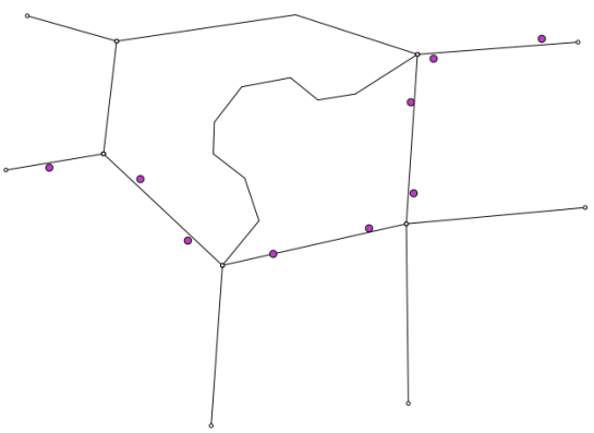
You can get a Spatialite file with testdata from Github as well. It contains a network and a routepoints1 layer:

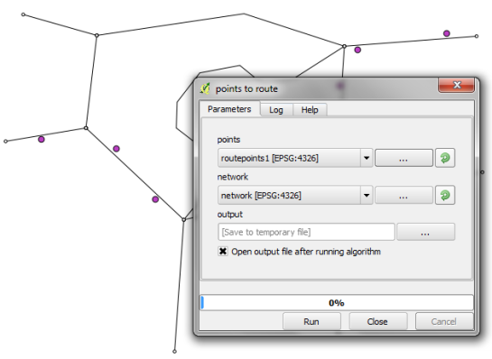
The interface of the points_to_route tool is very simple. All it needs as an input is information about which layer should be used as a network and which layer contains the route points:

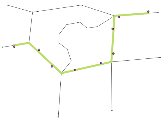
The input points are considered to be ordered. The tool always routes between consecutive points.

The result is a line layer with one line feature for each point pair:

The network analysis library is a really great new feature and I hope we will see a lot of tools built on top of it.

If you have to use IMRO data, you want to use the same legend as the one used on www.ruimtelijkeplannen.nl. Unfortunatly there is no standard IMRO legend file for QGIS. Luckily B3Partners uploaded an SLD file onto GitHub which you can use to create the legend in QGIS. To use the SLD for the legend […]

In the spirit of depesz’s “Waiting for Postgresql 9.#” series (and BostonGIS’ follow up Waiting for PostGIS 2.#), here’s the first in a new series of “Waiting for QGIS 2.2″ posts…

As I mentioned in my last post, one of my major goals for QGIS 2.2 is to make the print composer behave more like a professional DTP package. A big part of this is making sure QGIS respects all the expected standard behaviour for graphic design programs. While the print composer made huge advances toward this goal in version 2.0, there’s still further we can go.

So, let’s start with a list of all the new usability features the print composer has already gained for QGIS 2.2:

• Selections of multiple items can all be moved and resized together (previously only one item in the selection would be altered)
• Mouse handles are always drawn on the top of the composition – in earlier versions mouse handles could be hidden by items sitting higher in the composition
• Holding shift while resizing items locks their aspect ratio
• Holding control while resizing items causes them to resize from their centre
• Holding shift while moving items locks the movement to the horizontal or vertical
• Holding control while moving items temporarily disables any grid or guide-based snapping
• Items can be removed from a selection by shift-clicking them
• Control-clicking an item causes the next item below it to be selected – this allows you to select items which are hidden behind other items
• Holding shift while moving items using the cursor keys results in a large item movement
• There’s a new “Edit” menu in the composer, with options like
  • Select All/Select None and Invert Selection
  • Select Next Item Above and Select Next Item Below
  • Lock Selected Items and Unlock All

The new composer “Edit” menu

Additionally, there’s a bunch of pull requests which haven’t yet been merged to master, but are ready to go, including:

• Adding a dedicated “pan” tool for dragging around compositions
• Compositions can be panned at any time by holding the space key or middle mouse button
• Compositions can be zoomed by using the mouse wheel

Composer pan tool

Some of these are simple little changes which don’t sound like much, but it’s not until you’re forced to work without something like shift-resizing to lock the aspect ratio that you realise how often you use it and rely on it!

Last Sunday, the 6th of October, Eloise Woodrow was born by emergency caesarean. We had run into a few speed bumps along the way during the pregnancy so we knew there might be some issues when she was born. They had found she was small for her gestational age and also had a VSD (heart defect), this kind of thing, we didn't find out till later, can be linked to chromosomal issues. The most common issue being Downs Syndrome. There are also two other chromosomal issues, T13 and T18, both which have grim outcomes. It was fine, we told ourselves, we can live with a child with Downs, we have known and been friends with plenty of Downs children it wasn't really a concern. In the end the chance of T13 and T18 is so rare that it isn't going to happen to us. Well it was nice to believe that.

Yesterday our worst fear come true. Eloise has T18. The survival rate for babies with T18 is extremely low, and most don't make it past age one. They don't do the heart operation because of the poor survival rate. This means she has no chance and will die. Maybe in a few days, or weeks, but not months.

As a parent this is not something that we have ever wanted to deal with. Not so soon. Not ever. It's hard enough losing a friend or a relative let alone your own child. Every parent knows they would throw themselves under a bus for their children. If you could take the pain yourself and free them you would. But you can't and that makes it harder.

To the dumb question "Why me?" the cosmos barely bothers to return the reply: why not?

Christopher Hitchens

Not being a believer in any gods, or devine power, sometimes bad things just happen to good people for no reason. Others have to deal with this kind of pain so why not us too. We will get though it. We will try again.

The only solace that I can take from it all is that it's a (mostly) random event that no one could predict or prevent. It's not anyone's fault. Just a bad thing that happened.

For now the only thing we can do is be with her, love her, and make sure she is comfortable.

Mummy, Daddy, and Harry love you baby girl

Last Sunday, the 6th of October, Eloise Woodrow was born by emergency caesarean. We had run into a few speed bumps along the way during the pregnancy so we knew there might be some issues when she was born. They had found she was small for her gestational age and also had a VSD (heart defect), this kind of thing, we didn't find out till later, can be linked to chromosomal issues. The most common issue being Downs Syndrome. There are also two other chromosomal issues, T13 and T18, both which have grim outcomes. It was fine, we told ourselves, we can live with a child with Downs, we have known and been friends with plenty of Downs children it wasn't really a concern. In the end the chance of T13 and T18 is so rare that it isn't going to happen to us. Well it was nice to believe that.

Yesterday our worst fear come true. Eloise has T18. The survival rate for babies with T18 is extremely low, and most don't make it past age one. They don't do the heart operation because of the poor survival rate. This means she has no chance and will die. Maybe in a few days, or weeks, but not months.

As a parent this is not something that we have ever wanted to deal with. Not so soon. Not ever. It's hard enough losing a friend or a relative let alone your own child. Every parent knows they would throw themselves under a bus for their children. If you could take the pain yourself and free them you would. But you can't and that makes it harder.

To the dumb question "Why me?" the cosmos barely bothers to return the reply: why not?

Christopher Hitchens

Not being a believer in any gods, or devine power, sometimes bad things just happen to good people for no reason. Others have to deal with this kind of pain so why not us too. We will get though it. We will try again.

The only solace that I can take from it all is that it's a (mostly) random event that no one could predict or prevent. It's not anyone's fault. Just a bad thing that happened.

For now the only thing we can do is be with her, love her, and make sure she is comfortable.

Mummy, Daddy, and Harry love you baby girl

Last Sunday, the 6th of October, Eloise Woodrow was born by emergency caesarean. We had run into a few speed bumps along the way during the pregnancy so we knew there might be some issues when she was born. They had found she was small for her gestational age and also had a VSD (heart defect), this kind of thing, we didn't find out till later, can be linked to chromosomal issues. The most common issue being Downs Syndrome. There are also two other chromosomal issues, T13 and T18, both which have grim outcomes. It was fine, we told ourselves, we can live with a child with Downs, we have known and been friends with plenty of Downs children it wasn't really a concern. In the end the chance of T13 and T18 is so rare that it isn't going to happen to us. Well it was nice to believe that.

Yesterday our worst fear come true. Eloise has T18. The survival rate for babies with T18 is extremely low, and most don't make it past age one. They don't do the heart operation because of the poor survival rate. This means she has no chance and will die. Maybe in a few days, or weeks, but not months.

As a parent this is not something that we have ever wanted to deal with. Not so soon. Not ever. It's hard enough losing a friend or a relative let alone your own child. Every parent knows they would throw themselves under a bus for their children. If you could take the pain yourself and free them you would. But you can't and that makes it harder.

To the dumb question "Why me?" the cosmos barely bothers to return the reply: why not?

Christopher Hitchens

Not being a believer in any gods, or devine power, sometimes bad things just happen to good people for no reason. Others have to deal with this kind of pain so why not us too. We will get though it. We will try again.

The only solace that I can take from it all is that it's a (mostly) random event that no one could predict or prevent. It's not anyone's fault. Just a bad thing that happened.

For now the only thing we can do is be with her, love her, and make sure she is comfortable.

Mummy, Daddy, and Harry love you baby girl

I want to identify which areas of Chetney Marshes would be flooded by a 2m rise in sea level.  I used LIDAR data in contour format as the elevation data:-

Chetney Marshes map

Create TIN

I am using the TIN method to create an elevation model as the area is relatively small and the data is supplied as contours. TIN’s are more accurate, especially if the source data isn’t in grid format. However they are slower to process, especially over very large areas.

Select Plugins, Interpolation to open the Interpolation dialogue:-

I made the following changes to the display properties:-

• Colour map – Pusedocolour
• Transparency – I set global transparency to 50%

Chetney Marsh after colour adjustment

Raster Calculator

I now have an elevation model of the area. I now use the Raster Calculator to identify each pixel with an elevation of less than 2m. The elevation is stored in the pixel value. The raster calculator will identify each pixel with band value of less than 2.

The expression is elevation < 2

Select Raster, Raster Calculator to open the Raster Calculator:-

To change the Display Properties for a layer, Right click on the Layer in the layers panel (Table of Contents) and select Properties. I made the following changes to the display properties so the areas that are less than 2m, and susceptible to flooding appear highlighted in blue:-

• Style tab: Color map – Colormap
• Transparency: Global transparency 50%
• Colormap tab: I added 2 entries:-
  • 0.00 white
  • 1.00 blue

Chetney Marsh showing raster calculation results

In our first posting (“Processing Landsat 8 data in GRASS GIS 7: Import and visualization“) we imported a Landsat 8 scene (covering Raleigh, NC, USA). In this exercise we use Landsat data converted to reflectance with i.landsat.toar as shown in the first posting.

Here we will try color balancing and pan-sharpening, i.e. applying the higher resolution panchromatic channel to the color channels, using i.landsat.rgb.

1. Landsat 8 – RGB color balancing: natural color composites

After import, the RGB (bands 4,3,2 for Landsat 8) may look initially less exciting than expected.This is easy to fix by a histogram based auto-balancing of the RGB color tables.

To brighten up the RGB composite, we can use the color balancing tool of GRASS GIS 7:

As input, we specify the bands 4, 3, and 2:

Using a “Cropping intensity (upper brightness level)” of 99 (percent), the result look as follows:

For special purposes or under certain atmospheric/ground conditions it may be useful to make use of the functions “Preserve relative colors, adjust brightness only” or “Extend colors to full range of data on each channel” in the “Optional” tab of i.landsat.rgb.

You will need to experiment since the results depend directly on the image data.

2. Landsat 8 pansharpening

Pansharpening is a technique to merge the higher geometrical pixel resolution of the panchromatic band (Band 8) with the lower resolution color bands (Bands 4, 3, 2).

GRASS GIS 7 offers several methods through the command i.pansharpen.

1) Brovey transform:

This module runs in multi-core mode parallelized. The management of the resolution (i.e., apply the higher resolution of the panchromatic band) is performed automatically.

2. IHS transform

Here we select as above the bands in the i.pansharpen interface but use the “ihs” method.

HINT: If the colors should look odd, then apply i.landsat.rgb to the pan-sharpened bands (see above).

Color-adjusted IHS pansharpening (with “Cropping intensity: strength=99″):

Comparison of Landsat 8 RGB composite (39m) and IHS pansharpened RGB composite (15m):

3. PCA transform

Here we select as above the bands in the i.pansharpen interface but use the “pca” method.

Likewise other channels may be merged with i.pansharpen, even when originating from different sensors.

3. Conclusions

Overall, the IHS pansharpening method along with auto-balancing of colors appears to perform very well with Landsat 8.

Der OpenSource-Park auf der Intergeo wächst weiter! In diesem Jahr findet die Intergeo vom 8. bis 10. Oktober in Essen statt. Der OpenSource-Park befindet sich in Halle 1, Stand Nr. H1.033. Das OpenStreetMap Projekt ist mit dem Stand H1.040 gleich neben dem OpenSource-Park vertreten..

Auch auf der diesjährigen Hauptmesse der Geo-Informatik-Branche, der Intergeo, wird es wieder eine zentrale Anlaufstelle für alle Besucher geben, die sich über professionelle OpenSource-Anwendungen informieren wollen. Die Zahl der ausstellenden Firmen auf dem OpenSource-Park ist gegenüber dem Vorjahr nochmals um 50% angewachsen. Damit spiegelt die Messebeteiligung auch den über die Jahre stetig anwachsenden Marktanteil quelloffener Lösungen wieder. “Die Bedeutung von OpenSource-Software steigt nach unseren Beobachtungen von Jahr zu Jahr an”, bestätigt Projektleiter Daniel Katzer von der HINTE GmbH, die die INTERGEO für den DVW ausrichtet.

In diesem Jahr sind Firmen aus ganz Deutschland und der Schweiz auf dem OpenSource-Park vertreten. Die Schwerpunkte der ausstellenden Firmen liegen bei den Themen Performance-Optimierung für große Datenmengen, schnelle und umfassende Suchfunktionen über verteilte Datenbestände, Lösungen für die Ver- und Entsorgungsbranche, Geoportale für Unternehmen und Behörden, und natürlich im Bereich spezialisierter Beratungsleistungen.

Insgesamt steht damit auf dem OpenSource-Park ein Wissenspool zur Verfügung, der nicht nur alle gängigen Bereiche der räumlichen Datenverarbeitung umfasst, sondern daneben auch zahlreiche spezifische Themen und Branchenlösungen bereithält.

Der FOSSGIS e.V. versorgt Sie gerne mit Informationen rund um freie Software aus dem GIS Bereich und freie Geodaten. Zahlreiche Projekte sind über die OSGeo (Open Source Geospatial Foundation) vertreten. Es liegt Informationsmaterial für Sie bereit. Wir beraten Sie gerne!

Vortragsprogramm auf dem OpenSource-Park

Ein Highlight wird wie jedes Jahr das umfangreiche Vortragsprogramm an allen drei Tagen sein. Es erwarten Sie u.a. Vorträge zu OpenStreetMap, QGIS, INSPIRE, D115, ALKIS, Cloud-Diensten, Bürgerbeteiligungssystemen, diversen Fachschalen und vielen weiteren Neuerungen und Best-Practice-Beispielen.

Das Vortragsprogramm wird vom FOSSGIS e.V. organisiert.

Ausstellende Firmen

Ausstellende Firmen auf dem diesjährigen OpenSource-Park der Intergeo:

• Mapwebbing
• Metaspatial
• norBIT GmbH
• Omniscale GmbH & Co. KG
• rasdaman GmbH/ Jacobs University Bremen
• Sourcepole AG
• terrestris GmbH & Co. KG
• WebGis - in medias res GmbH
• WhereGroup GmbH & Co. KG

OSM Stand

Das OpenStreetMap Projekt ist in diesem Jahr mit einem eigenen Stand auf der Intergeo vertreten. Dieser grenzt direkt an den OSGeo Park an und befindet sich in Halle 1, Stand Nr. H1.040. Schauen Sie doch vorbei und informieren Sie sich über die neusten Entwicklungen im OpenStreetMap-Projekt.

Rahmenprogramm

OSM Stammtisch im Unperfekthaus

Im Rahmen des Engagements des FOSSGIS e.V. auf der INTERGEO 2013 findet am 08.10.2013 ab 19 Uhr der OSM Stammtisch im Unperfekthaus , Essen statt.

FOSSGIS e.V. Vollversammlung

Am 09.10.2013 trifft sich der FOSSGIS e.V. zur Vollversammlung auf der Intergeo.

Wir freuen uns auf Ihren Besuch auf der Intergeo. Schauen Sie doch auf dem OpenSource-Park vorbei!

Der OpenSource-Park auf der Intergeo wächst weiter! In diesem Jahr findet die Intergeo vom 8. bis 10. Oktober in Essen statt. Der OpenSource-Park befindet sich in Halle 1, Stand Nr. H1.033. Das OpenStreetMap Projekt ist mit dem Stand H1.040 gleich neben dem OpenSource-Park vertreten..

Auch auf der diesjährigen Hauptmesse der Geo-Informatik-Branche, der Intergeo, wird es wieder eine zentrale Anlaufstelle für alle Besucher geben, die sich über professionelle OpenSource-Anwendungen informieren wollen. Die Zahl der ausstellenden Firmen auf dem OpenSource-Park ist gegenüber dem Vorjahr nochmals um 50% angewachsen. Damit spiegelt die Messebeteiligung auch den über die Jahre stetig anwachsenden Marktanteil quelloffener Lösungen wieder. “Die Bedeutung von OpenSource-Software steigt nach unseren Beobachtungen von Jahr zu Jahr an”, bestätigt Projektleiter Daniel Katzer von der HINTE GmbH, die die INTERGEO für den DVW ausrichtet.

In diesem Jahr sind Firmen aus ganz Deutschland und der Schweiz auf dem OpenSource-Park vertreten. Die Schwerpunkte der ausstellenden Firmen liegen bei den Themen Performance-Optimierung für große Datenmengen, schnelle und umfassende Suchfunktionen über verteilte Datenbestände, Lösungen für die Ver- und Entsorgungsbranche, Geoportale für Unternehmen und Behörden, und natürlich im Bereich spezialisierter Beratungsleistungen.

Insgesamt steht damit auf dem OpenSource-Park ein Wissenspool zur Verfügung, der nicht nur alle gängigen Bereiche der räumlichen Datenverarbeitung umfasst, sondern daneben auch zahlreiche spezifische Themen und Branchenlösungen bereithält.

Der FOSSGIS e.V. versorgt Sie gerne mit Informationen rund um freie Software aus dem GIS Bereich und freie Geodaten. Zahlreiche Projekte sind über die OSGeo (Open Source Geospatial Foundation) vertreten. Es liegt Informationsmaterial für Sie bereit. Wir beraten Sie gerne!

Vortragsprogramm auf dem OpenSource-Park

Ein Highlight wird wie jedes Jahr das umfangreiche Vortragsprogramm an allen drei Tagen sein. Es erwarten Sie u.a. Vorträge zu OpenStreetMap, QGIS, INSPIRE, D115, ALKIS, Cloud-Diensten, Bürgerbeteiligungssystemen, diversen Fachschalen und vielen weiteren Neuerungen und Best-Practice-Beispielen.

Das Vortragsprogramm wird vom FOSSGIS e.V. organisiert.

Ausstellende Firmen

Ausstellende Firmen auf dem diesjährigen OpenSource-Park der Intergeo:

• Mapwebbing
• Metaspatial
• norBIT GmbH
• Omniscale GmbH & Co. KG
• rasdaman GmbH/ Jacobs University Bremen
• Sourcepole AG
• terrestris GmbH & Co. KG
• WebGis - in medias res GmbH
• WhereGroup GmbH & Co. KG

OSM Stand

Das OpenStreetMap Projekt ist in diesem Jahr mit einem eigenen Stand auf der Intergeo vertreten. Dieser grenzt direkt an den OSGeo Park an und befindet sich in Halle 1, Stand Nr. H1.040. Schauen Sie doch vorbei und informieren Sie sich über die neusten Entwicklungen im OpenStreetMap-Projekt.

Rahmenprogramm

OSM Stammtisch im Unperfekthaus

Im Rahmen des Engagements des FOSSGIS e.V. auf der INTERGEO 2013 findet am 08.10.2013 ab 19 Uhr der OSM Stammtisch im Unperfekthaus , Essen statt.

FOSSGIS e.V. Vollversammlung

Am 09.10.2013 trifft sich der FOSSGIS e.V. zur Vollversammlung auf der Intergeo.

Wir freuen uns auf Ihren Besuch auf der Intergeo. Schauen Sie doch auf dem OpenSource-Park vorbei!

For our analysis example, we’ll obtain (freely – thanks, NASA and USGS!) a Landsat 8 scene from http://earthexplorer.usgs.gov/

First of all, you should register.

1. Landsat 8 download procedure

1. Enter Search Criteria:

• path/row tab, enter Type WRS2: Path: 16, Row: 35
• Date range: 01/01/2013 – today
• Click on the “Data sets >>” button

2. Select Your Data Set(s):

• Expand the entry + Landsat Archive
      [x] L8 OLI/TIRS
• Click on the “Results >>” button

(We jump over the additional criteria)

4. Search Results

From the resulting list, we pick the data set:

Entity ID: LC80160352013134LGN03
Coordinates: 36.04321,-79.28696
Acquisition Date: 14-MAY-13

Using the “Download options”, you can download the data set (requires login). Select the choice:
[x] Level 1 GeoTIFF Data Product (842.4 MB)

You will receive the file “LC80160352013134LGN03.tar.gz”.

2. Unpacking the downloaded Landsat 8 dataset

To unpack the data, run (or use a graphical tool at your choice):

tar xvfz LC80160352013134LGN03.tar.gz

A series of GeoTIFF files will be extracted: LC80160352013134LGN03_B1.TIF, LC80160352013134LGN03_B2.TIF, LC80160352013134LGN03_B3.TIF, LC80160352013134LGN03_B4.TIF, LC80160352013134LGN03_B5.TIF, LC80160352013134LGN03_B6.TIF, LC80160352013134LGN03_B7.TIF, LC80160352013134LGN03_B8.TIF, LC80160352013134LGN03_B9.TIF, LC80160352013134LGN03_B10.TIF, LC80160352013134LGN03_B11.TIF, LC80160352013134LGN03_BQA.TIF

We may check the metadata with “gdalinfo“:

gdalinfo LC80160352013134LGN03_B1.TIF
Driver: GTiff/GeoTIFF
Files: LC80160352013134LGN03_B1.TIF
Size is 7531, 7331
Coordinate System is:
PROJCS["WGS 84 / UTM zone 17N",
    GEOGCS["WGS 84",
        DATUM["WGS_1984",
            SPHEROID["WGS 84",6378137,298.257223563,
...
Pixel Size = (30.000000000000000,-30.000000000000000)
...

3. Want to spatially subset the Landsat scene first?

If you prefer to cut out a smaller area (subregion), check here for gdal_translate usage examples.

4. Import into GRASS GIS 7

Note: While this Landsat 8 scene covers the area of the North Carolina (NC) sample dataset, it is delivered in UTM rather than the NC's state plane metric projection. Hence we preprocess the data first in its original UTM projection prior to the reprojection to NC SPM.

Using the Location Wizard, we can import the dataset easily into a new location (in case you don't have UTM17N not already created earlier):

grass70 -gui

Now start GRASS GIS 7 and you will find the first band already imported (the others will follow shortly!).

For the lazy folks among us, we can also create a new GRASS GIS Location right away from the dataset on command line:

grass70 -c LC80160352013134LGN03_B10.TIF ~/grassdata/utm17n

5. Importing the remaining Landsat 8 bands

The remaining bands can be easily imported with the raster import tool:

The bands can now be selected easily for import:

• Select "Directory" and navigate to the right one
• The available GeoTIFF files will be shown automatically
• Select those you want to import
• You may rename (double-click) the target name for each band
• Extend the computation region accordingly automatically

Click on "Import" to get the data into the GRASS GIS location. This takes a few minutes. Close the dialog window then.

In the "Map layers" tab you can select the bands to be shown:

6. The bands of Landsat 8

(cited from USGS)

Landsat 8 Operational Land Imager (OLI) and Thermal Infrared Sensor (TIRS) images consist of nine spectral bands with a spatial resolution of 30 meters for Bands 1 to 7 and 9. New band 1 (ultra-blue) is useful for coastal and aerosol studies. New band 9 is useful for cirrus cloud detection. The resolution for Band 8 (panchromatic) is 15 meters. Thermal bands 10 and 11 are useful in providing more accurate surface temperatures and are collected at 100 meters. Approximate scene size is 170 km north-south by 183 km east-west (106 mi by 114 mi).

* TIRS bands are acquired at 100 meter resolution, but are resampled to 30 meter in delivered data product.

7. Natural color view (RGB composite)

Due to the introduction of a new "Cirrus" band (#1), the BGR bands are now 2, 3, and 4, respectively. See also "Common band combinations in RGB" for Landsat 7 or Landsat 5, and Landsat 8.

From Digital Numer (DN) to reflectance:
Before creating an RGB composite, it is important to convert the digital number data (DN) to reflectance (or optionally radiance). Otherwise the colors of a "natural" RGB composite do not look convincing but rather hazy (see background in the next screenshot). This conversion is easily done using the metadata file which is included in the data set with i.landsat.toar:

Now we are ready to create a nice RGB composite:

Select the bands to be visually combined:

... and voilà!

8. Applying the Landsat 8 Quality Assessment (QA) Band

One of the bands of a Landsat 8 scene is named "BQA" which contains for each pixel a decimal value representing a bit-packed combination of surface, atmosphere, and sensor conditions found during the overpass.  It can be used to judge the overall usefulness of a given pixel.

We can use this information to easily eliminate e.g. cloud contaminated pixels. In short, the QA concept is (cited here from the USGS page):

For the single bits (0, 1, 2, and 3):
0 = No, this condition does not exist
1 = Yes, this condition exists.

The double bits (4-5, 6-7, 8-9, 10-11, 12-13, and 14-15) represent levels of confidence that a condition exists:
00 = Algorithm did not determine the status of this condition
01 = Algorithm has low confidence that this condition exists (0-33 percent confidence)
10 = Algorithm has medium confidence that this condition exists (34-66 percent confidence)
11 = Algorithm has high confidence that this condition exists (67-100 percent confidence).

Detailed bit patterns (d: double bits; s: single bits):
d  Bit 15 = 0 = cloudy
d  Bit 14 = 0 = cloudy
d  Bit 13 = 0 = not a cirrus cloud
d  Bit 12 = 0 = not a cirrus cloud
d  Bit 11 = 0 = not snow/ice
d  Bit 10 = 0 = not snow/ice
d  Bit 9 = 0 = not populated
d  Bit 8 = 0 = not populated
d  Bit 7 = 0 = not populated
d  Bit 6 = 0 = not populated
d  Bit 5 = 0 = not water
d  Bit 4 = 0 = not water
s  Bit 3 = 0 = not populated
s  Bit 2 = 0 = not terrain occluded
s  Bit 1 = 0 = not a dropped frame
s  Bit 0 = 0 = not fill

Usage example 1:  Creating a mask from a bitpattern

We can create a cloud mask (bit 15+14 are set) from this pattern:
cloud:   1100000000000000

Using the Python shell tab, we can easily convert this into the corresponding decimal number for r.mapcalc:

Welcome to wxGUI Interactive Python Shell 0.9.8

Type "help(grass)" for more GRASS scripting related information.
Type "AddLayer()" to add raster or vector to the layer tree.

Python 2.7.5 (default, Aug 22 2013, 09:31:58) 
[GCC 4.8.1 20130603 (Red Hat 4.8.1-1)] on linux2
Type "help", "copyright", "credits" or "license" for more information.
>>> int(0b1100000000000000)
49152

Using this decimal value of 49152, we can create a cloud mask:

# set NULL for cloudy pixels, 1 elsewhere:
r.mapcalc "cloudmask = if(LC80160352013134LGN03_BQA == 49152, null(), 1 )"

# apply this mask
r.mask cloudmask

In our sample scene, there are only tiny clouds in the north-east, so no much to be seen. Some spurious cloud pixels are scattered over the scene, too, which could be eliminated (in case of false positives) or kept.

Usage example 2:  Querying the Landsat 8 BQA map and retrieve the bitpattern

Perhaps you prefer to query the BQA map itself (overlay the previously created RGB composite and query the BSA map by selecting it in the Layer Manager). In our example, we query the BQA value of the cloud:

Using again the Python shell tab, we can easily convert the decimal number (used for r.mapcalc) into the corresponding binary representation to verify with the  table values above.

>>> x=61440
>>> print(bin(x & 0xffffffff))
0b1111000000000000

Hence, bits 15,14,13, and 12 are set: cloudy and not a cirrus cloud. Looking at the RGB composite we tend to agree Time to mask out the cloud!

wxGUI menu >> Raster >> Mask [r.mask]

Or use the command line, as shown already above:

# remove existing mask (if active)
r.mask -r

# set NULL for cloudy pixels, 1 elsewhere:
r.mapcalc "cloudmask = if(LC80160352013134LGN03_BQA == 61440, null(), 1 )" --o

# apply the new mask
r.mask cloudmask

The visual effect in the RGB composite is minimal since the cloud is white anyway (as NULL cells, too). However, it is relevant for real calculations such as NDVI (vegetation index) or thermal maps.

We observe dark pixels around the cloud originating from thin clouds. In a subsequent identification/mask step we may eliminate also those pixels with a subsequent filter.