One of the big features I worked on for QGIS 2.2 is gradient fill symbols for polygons. In my view QGIS’ symbol support is one of its biggest strengths — the versatility of its symbol layers coupled with the powerful data defined properties support allows for so many effects which just aren’t possible in other GIS packages. Gradient fill support is a nice addition to these features and should help make QGIS even more attractive to cartographers. In this post I’m going to give a quick run through of how gradient fills work in QGIS, and some of the options available for tweaking them.

Gradient fills are enabled through the Style tab in the properties for a vector layer. The default fill for a polygon in QGIS is “Simple fill”, so to switch a layer to a gradient fill you first need to select the “Simple fill” layer, then change the “Symbol layer type” dropdown  to “Gradient fill”:

As you can see, there’s a lot of options in QGIS which can be tweaked for gradient fills. I’ll run through each of them now and explain a little bit about how each one can be used.

Colour modes

QGIS supports two different types of colour modes for gradient fills. The first is a simple “Two color” gradient, where the colour smoothly blends from the first colour to the second. The second mode, “Color ramp” allows you to use any of the standard or user-defined QGIS colour ramps, which can consist of multiple colour stops:

Colour options in gradient fills

So, when would you use these options? Well, any time you need more than two colours or need to tweak the position of any of the colours in the gradient you’ll have to use a colour ramp.  If instead you’re just wanting a quick-and-easy gradient then the two colour option might be more suitable.

One last important distinction is that the colours in a two colour gradient can be set using a data defined expression:

Data defined gradient colours. Please try to use them more tastefully then this!

Gradient types

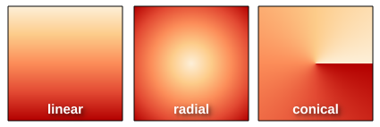
The next option for gradient fills is rather self-explanatory: gradient types. QGIS supports linear, radial and conical gradients:

Coordinate modes

The coordinate mode option is a little trickier to explain. The default setting, “Object“, will cause the gradient to be drawn entirely within each separate feature. You can see in the example below that every lake feature is coloured with a gradient which starts with light blue in the top left and darkens to a deeper blue in the bottom right. This gradient fill is repeated for all the lake features:

The “Object” coordinate mode for gradient fills

In contrast, the “Viewport” coordinate mode causes the gradient to be drawn across the entire current view of the map. So only the lakes in the top left of the map are drawn with the light blue colour, and the lakes in the bottom right with the deeper blue:

The “Viewport” coordinate mode for gradient fills

The choice of coordinate mode will depend entirely on your cartographic desires for your map!

Reference points

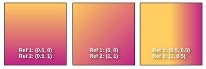
QGIS gradient fills allow the setting of two “reference points“. These points control where the gradient fill begins and ends. It’s easiest to visualise how these work by imagining a square defined by the points (0, 0) in the top left and (1, 1) in the bottom right. The two reference points fall somewhere within this square. So, the default reference points of (0.5, 0) and (0.5, 1.0) represent points mid way along the top edge and and the bottom edge, respectively.

Now imagine that this square forms the bounding box for the feature being drawn (or the current map window, if in “viewport” coordinate mode). The default reference points mean that the gradient will be drawn from the middle of the top edge to middle of the bottom edge of the feature. Reference points of (0, 0) and (1, 1) would mean the gradient is drawn from the top-left to the bottom-right. Similarly, reference points of (0.5, 0.5) to (1.0, 1.0) would draw a gradient from the middle of the feature to the bottom right (good for radial gradients).

There’s also the option to set either of the reference points as the feature centroid, which again can come in handy for radial or conical gradient types.

Gradient spread

If you’ve got your head around the reference points concept, then the next setting for gradient fills affects how the gradients spread. This takes effect whenever a gradient starts or ends before the bounds of the feature. The default setting of “pad” means that the gradient will simple “pad” out any extra space with the start or end gradient colour:

“Pad” spread – notice how the darker blue is stretched across the right side of each feature

“Repeat” mode will tile the gradient across the feature:

“Repeat” spread

Finally, “reflect” mode will draw a reflected version of the gradient to fill up any extra space:

“Reflect” spread

Angle

Last of all, there’s a simple “angle” parameter, which allows you to rotate the entire gradient fill. This option is included mostly for use with data defined symbols, since a similar effect can be achieved by changing the gradient reference points. Amongst other effects, this is useful for achieving a “sun glint” on water, where each gradient is drawn in a random direction (more on this in a later blog post):

Random data defined gradient angles

This leads me into my final note… all of these properties can be data defined! So you could have a column in your data controlling whether each feature is drawn with a radial or linear gradient, or whether the gradient in a given feature should be drawn at a specific angle, or that the gradient in a feature should start at the centroid and end at the top right of the feature!

I’m excited to see what the QGIS user community is able to create using this new gradient fill feature when 2.2 is released. If you’ve already had a chance to play with the dev version of 2.2 and have something to show off, make sure you submit your map to the Flickr QGIS Map Showcase!

A Faunalia, em colaboração com a ENCPB (Escola Nacional de Caça, Pesca e Biodiversidade), Comoiprel e Câmara Municipal de Moura, organiza um curso de SIG Open Source com QGIS (Quantum GIS) nos dias 17-18-19 Março 2014. Data limite para inscrições: 3 de Março. Para informações e inscrições contactar: ENCPB (Escola Nacional de Caça, Pesca e […]

and thank you for a great 2013!

It has been a very busy year between writing my first book, going to FOSS4G, writing my first journal article and continuing to write this blog. The blog view counter shows a staggering 310,000 views for 2013.

The most popular posts of 2013 were:

1. pgRouting 2.0 for Windows quick guide
2. Vintage map design using QGIS
3. Group Stats tutorial
4. the Print Composer 2.0 series
5. and Public transport isochrones with pgRouting

All the best for 2014!

OSM place search and osmSearch are two plugins for QGIS which use the Nominatim service to find addresses and places. They are both still marked as “experimental” plugins, so users are expected to expect the unexpected.

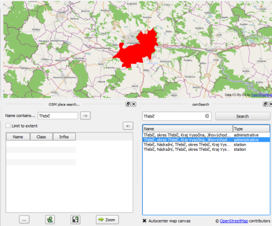
Once installed, both plugins look very similar: There is an input text field and a results list.

A simple search with street name and house number returns the expected results. Interacting with the result shows some differences:

• OSM place search will highlight the location when you mouse-over the result in the list. On double-click, it will zoom to the result.
• osmSearch will highlight the result and move the map center to the result if you double-click but won’t zoom.

Both plugins can deal with umlauts (ä,ö,ü) but only osmSearch works with háčeks.

A nice feature of osmSearch is that it remembers your previous searches and offers an auto-complete function.

OSM place search on the other hand offers a reverse “Where am I” function (the arrow pointing to the left” which tries to find a name for the current map center location. Additionally, there are functions to add the current object as a new layer or mask layer.

Both plugins have strong and weak points. Combined, they would make a really strong tool but then nothing prevents us from having them both and choosing the best one for the task at hand.

Recently, in order to nicely plan ahead for a birthday lunch at the agritur Malga Brigolina (a farm-restaurant near Sopramonte di Trento, Italy, at 1,000m a.s.l. in the Southern Alps), friends of mine asked me the day before:

“Will the place be sunny at lunch time for a nice walk?“

[well, the weather was close to clear sky conditions but mountains are high here and casting long shadows in the winter time].

A rather easy task I thought, so I got my tools ready since that was an occasion to verify the predictions with some photos! Thanks to the new EU-DEM at 25m I was able to perform the computations right away in a metric system rather than dealing with degree in LatLong.

Direct sunlight can be assessed from the beam radiation map of GRASS GIS’ r.sun when running it for a specific day and time. But even easier, there is a new Addon for GRASS GIS 7 which calculates right away time series of insolation maps given start/stop timestamps and a time step: r.sun.hourly. This shrinks the overall effort to almost nothing.

1. Creating the direct sunlight maps

The first step is to calculate where direct sunlight reaches the ground. Here the input elevation map is the European “eu_dem_25″, while the output is the beam radiation for a certain day (15 Dec 2013 is DOY 349).

Important hint: the computational region must be large enough to east/south/west to capure the cast shadow effects of all relevant surrounding mountains.

I let calculations start at 8am and finish at 5pm which an hourly time step. The authors have kindly parallelized r.sun.hourly, so I let it run on four processors simultaneously to speed up:

# calculate DOY (day-of-year) from given date:
date -d 2013-12-15 +%j
349

# calculate beam radiation maps for a given time period
# (note: minutes are to be given in decimal time: 30min = 0.5)
r.sun.hourly elev_in=eu_dem_25 beam_rad=trento_beam_doy349 \
      start_time=8 end_time=17 time_step=1 day=349 year=2013 \
      nprocs=4

The ten resulting maps contain the beam radiation for each pixel considering the cast shadow effects of the pixel-surrounding mountains. However, the question was not to calculate irradiance raster maps in Wh/m^2 but simply “sun-yes” or “sun-no”. So a subsequent filtering had to be applied. Each beam radiation map was filtered: if pixel value equal to 0 then “sun-no”, otherwise “sun-yes” (what my friends wanted to achieve; effectively a conversion into a binary map).
Best done in a simple shell script loop:

[Edit 30 Dec 2013: thanks to Anna you can simplify below loop to the r.colors call thanks to the new -b flag for binary output in r.sun.hourly!]

for map in `g.mlist rast pattern="trento_beam_doy349*"` ; do
    # rename current map to tmp
    g.rename rast=$map,$map.tmp
    # filter and save with original name
    r.mapcalc "$map = if($map.tmp == 0, null(), 1)"
    # colorize the binary map
    echo "1 yellow" | r.colors $map rules=-
    # remove cruft
    g.remove rast=$map.tmp
done

As a result we got ten binary maps, ideal for using them as overlay with shaded DEMs or OpenStreetMap layers. The areas exposed to direct sunlight are shown in yellow.

Trento, direct sunlight, 15 Dec 2013 between 10am and 5pm (See here for creating an animated GIF). Quality reduced for this blog.

2. Time to look at some details: So, is Malga Brigolina in sunlight at lunch time?

Situation at 12pm (noon): predicted that the restaurant is still in shadow – confirmed in the photo:

(click to enlarge)

Situation at 1:30/2:00pm: sun is getting closer to the Malga, as confirmed in photo (note that the left photo is 20min ahead of the map). The small street in the right photo is still in the shadow as predicted in the map):

(click to enlarge)

Situation at 3:00pm: sun here and there at Malga Brigolina:

Sunlight map blended with OpenStreetmap layer (r.blend + r.composite) and draped over DEM in wxNVIZ of GRASS GIS 7 (click to enlarge). The sunday walk path around Malga Brigolina is the blue/red vector line shown in the view center.

Situation at 4:00pm: we are close to sunset in Trentino… view towards the Rotaliana (Mezzocorona, S. Michele all’Adige), last sunlit summits also seen in photo:

(click to enlarge)

3. Outcome

The resulting sunlight/shadow map appear to match nicely realty. Perhaps r.sun.hourly should get an additional flag to generate the binary “sun-yes” – “sun-no” maps directly.

Direct sunlight zones (yellow, 15 Dec 2013, 3pm): Trento with Monte Bondone, Paganella, Marzolan, Lago di Caldonazzo, Lago di Levico and surroundings (click to enlarge)

4. GRASS GIS usage note

The wxGUI settings were as simple as this (note the transparency values for the various layers):

Data sources:

• Shaded maps produced using Copernicus data and information funded by the European Union – EU-DEM layers
• © OpenStreetMap contributors

The post Will the sun shine on us? appeared first on GFOSS Blog | GRASS GIS Courses.

Profile Tool is a plugin for QGIS which makes it possible to generate (elevation) profiles for line features. The plugin is available through the default QGIS plugin repository. While testing the plugin, I found some aspects of using the tool might require additional instructions.

After installing and enabling the plugin, you will find the “Terrain profile” button in the plugin toolbar:

The basic use case is as follows:

1. Load the elevation raster and select this raster layer in the layer list.
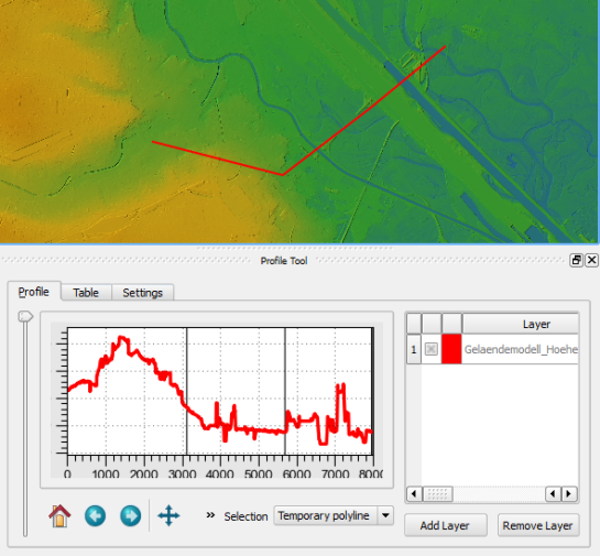
2. Press the “Terrain profile” button. This opens the plugin panel which consists of a graph area on the left and a raster layer list on the right. The raster layer you had selected will be added to the raster layer list.
3. If you have “Selection: Temporary polyline” enabled, you can now draw a line in the map area. Double-click left to end drawing the line. (If you are paying close attention, you might have noticed the instructions in the status bar.)
4. After you have finished drawing the line, the graph area will update and display the profile.

If you want to add another raster layer to the plugin, you need to first select the raster layer in the QGIS layer list and then press the “Add Layer” button in the Profile Tool panel.

To generate the profile for an existing line feature, you need to change the selection mode from “Temporary polyline” to “Selected polyline”. Then you need to select the vector layer which contains the line feature you want to use in the QGIS layer list. Finally, you can click on the line feature in the map area to select it. (Note that this selection is independent of any selections you might have going on using the default QGIS feature selection tools.)

If you change from the Profile Tool to any other tool such as “Pan Map” or “Identify”, you have to click the “Terrain profile” button again to re-enable drawing/selection a line for the Profile Tool.

Due to a bug, it is currently not possible to export the profile graph. An alternative is to open the “Table” tab of the Profile Tool panel which provides access to the profile data and copy the data into your preferred graphing application such as Calc or Excel.

If you want to see the Profile Tool in action, I recommend watching the introduction video by Lene Fischer (University of Copenhagen).

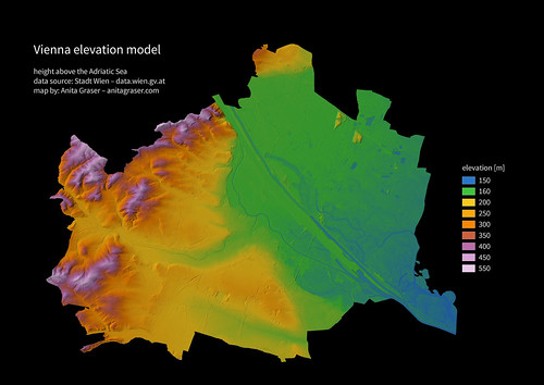
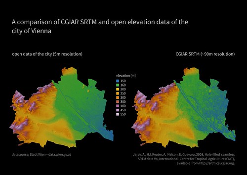
Since I finally managed to download the elevation model of the city of Vienna, I thought I’d share some eye candy with you: The map uses layer blending to combine hillshade and elevation raster, and the elevation raster’s color ramp is a modified “garish14″ from QGIS’ cpt-city color ramp collection.

wien_elevation, a photo by underdarkGIS on Flickr.

A comparion of CGIAR SRTM and open elevation data from the city of Vienna, a photo by underdarkGIS on Flickr.

Update

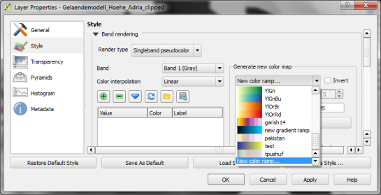
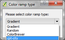
Here is how you get access to the “garish14″ color ramp:

Start by selecting the “new color ramp” option in the raster’s style window.

Chose the “cpt-city” color ramp type.

In the “cpt-city color ramp” window, you will find lots of different premade color ramps. “garish14″ is part of the “Topography” collection.

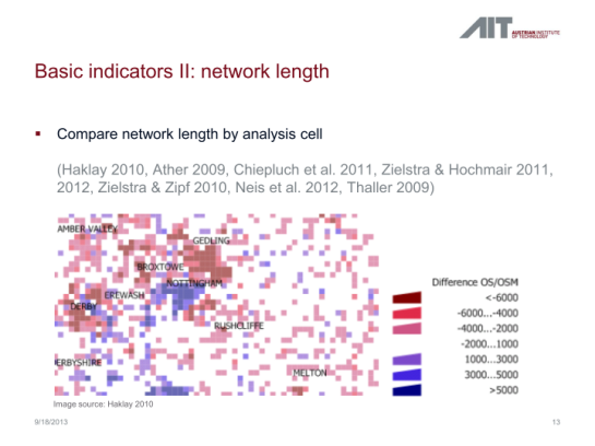
In my previous post, I presented a Processing model to determine positional accuracy of street networks. Today, I’ll cover another very popular tool to assess OSM quality in a region: network length comparison. Here’s the corresponding slide from my FOSS4G presentation which shows an example of this approach applied to OSM and OS data in the UK:

One building block of this tool is the Total graph length model which calculates the length of a network within specified regions. Like the model for positional accuracy, this model includes reprojection steps to ensure all layers are in the same CRS before the actual geoprocessing starts:

The final Compare total graph length model combines two instances of “Total graph length” whose results are then joined to eventually calculate the length difference (lenDIFF).

As usual, you can find the models on Github. If you have any questions, don’t hesitate to ask in the comments and if you find any issues please report them on Github.

The city of Winterthur recently launched their new public map portal, based on Mapfish Appserver. Some of the features are outlined in the online help (in German).

Mobile users are redirected to the OL3 Mobile Viewer, which is based on OpenLayers 3 and jQuery Mobile. To have a look at it from your desktop browser follow this link.

In contrary to the desktop version, most of the background layers are delivered as tiles and only topic layers are full size WMS requests. The interesting thing is, that instead of using a tile protocol like WMTS, TMS, etc., an OL3 tiled WMS datasource does multiple WMS requests in a tile scheme. The usual tiling problems (labels, etc.) do not apply for the used raster layers and Varnish serves as cache for on-the-fly generated WMS tiles. In contrary to file based tile caching, much less disk space and more important, no update process is needed.

@PirminKalberer

The city of Winterthur recently launched their new public map portal, based on Mapfish Appserver. Some of the features are outlined in the online help (in German).

Mobile users are redirected to the OL3 Mobile Viewer, which is based on OpenLayers 3 and jQuery Mobile. To have a look at it from your desktop browser follow this link.

In contrary to the desktop version, most of the background layers are delivered as tiles and only topic layers are full size WMS requests. The interesting thing is, that instead of using a tile protocol like WMTS, TMS, etc., an OL3 tiled WMS datasource does multiple WMS requests in a tile scheme. The usual tiling problems (labels, etc.) do not apply for the used raster layers and Varnish serves as cache for on-the-fly generated WMS tiles. In contrary to file based tile caching, much less disk space and more important, no update process is needed.

@PirminKalberer

Watch how the community based GRASS GIS 6.4 software development evolved! You can see how the individual contributors modify and expand the source code:

• Dec 29, 1999: GRASS GIS 5.0 is being stored in an online source code repository in December 1999…
• Dec 02, 2000: The developers work on all parts of the code…
• Jan 15, 2002: Working on the future GRASS GIS 5.1 release
• Nov 25, 2002: Starting GRASS 5.1 development with code restructuring
• Jun 14, 2004: GRASS GIS 5.7 released in June 2004
• Nov 09, 2004: Source code restructuring to get a better directory layout (all other developers waiting…)
• Nov 09, 2004: … thousands of files are modified in this operation …
• Nov 10, 2004: All developers resume their activities after the restructuring
• Jan 10, 2005: Preparing the GRASS GIS 6.0.0 release…
• Apr 09, 2005: GRASS GIS 6.0.0 published, release branch being split off from trunk for easier maintenance
• Feb 22, 2006: Release of GRASS GIS 6.0.2 and new source code refactoring startedApr 05, 2006: Heavy development activity in trunk (development branch) …
• Oct 25, 2006: GRASS GIS 6.2.0 released in October 2006
• Apr 10, 2007: Preparing the GRASS GIS 6.2.2 release…
• Jun 16, 2007: GRASS GIS 6.2.2 released in June 2007
• Nov 01, 2007: Raster and vector modules being actively maintained…
• Apr 02, 2007: New graphical user interface development speeding up (wxGUI)
• Feb 20, 2008: Copyright statements prettified in many files
• May 31, 2008: New GRASS 6 development branch being split off from trunk (which becomes GRASS 7)
• Jun 10, 2008: Developers moving over to new branch
• Feb 23, 2009: GRASS 6.4 release branch split off from GRASS 6 development branch
• Apr 03, 2009: GRASS GIS 6.4 preparations starting…
• Feb 24, 2010: Intense maintenance in GRASS 6.4 release branch
• Sep 15, 2010: GRASS GIS 6.4.0 released in September 2010
• Apr 12, 2011: GRASS GIS 6.4.1 released in April 2011
• Jun 27, 2011: GRASS GIS 6.4.svn matures for the upcoming 6.4.2 release
• Aug 16, 2011: Intense maintenance in GRASS 6.4 release branch (GRASS GIS 7 development not shown here)…
• Feb 19, 2012: GRASS GIS 6.4.2 released in February 2012
• Nov 13, 2012: Backporting graphical user interface bugfixes from GRASS GIS 7 to GRASS GIS 6.4
• Apr 17, 2013: Further maintenance in GRASS 6.4 release branch
• Jul 10, 2013: Fixing odds ‘n ends for the new stable release
• Jul 27, 2013: GRASS GIS 6.4.3 released in July 2013

The corresponding timeline is also available at
http://grass.osgeo.org/home/history/releases/

THANKS TO ALL CONTRIBUTORS!
http://grass.osgeo.org/development/

Rendering: Markus Neteler
Audio track editing: Duccio Rocchini & Antonio Galea

Music:
Le bruit peut rendre sourd – Track 6/18 Album “Sensation electronique” by Saelynh (CC-BY-NC-ND) http://www.jamendo.com/en/track/1236/le-bruit-peut-rendre-sourd

Software used:
Gource software: http://code.google.com/p/gource/ (GPL)
OpenShot video editor: http://www.openshotvideo.com/ (GPL

The post Video: GRASS GIS development visualization from 1999 to 2013 appeared first on GFOSS Blog | GRASS GIS Courses.

Over the last years, research on OpenStreetMap data quality has become increasingly popular. At this year’s FOSS4G, I had the honor to present some work we did at the AIT to assess OSM quality in Vienna, Austria. In the meantime, our paper “Towards an Open Source Analysis Toolbox for Street Network Comparison” has been published for early access. Thanks to the conference organizers who made this possible! I’ve implemented comparison tools found in related OSM literature as well as new tools for oneway street and turn restriction comparison using Sextante scripts and models for QGIS 1.8. All code is available on Github to enable collaboration. If you are interested in OSM data quality research, I’d like to invite you to give the tools a try.

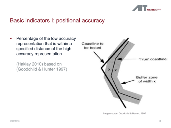
Since most users probably don’t have access to QGIS 1.8 anymore, I’ll be updating the tools to QGIS 2.0 Processing. I’m starting today with the positional accuracy comparison tool. It is based on a method described by Goodchild & Hunter (1997). Here’s the corresponding slide from my FOSS4G presentation:

The basic idea is to evaluate the positional accuracy of a street graph by comparing it with a reference graph. To do that, we check how much of the graph lies within a certain tolerance (buffer) of the reference graph.

The processing model uses the following input: the two street graphs which should be compared, the size of the buffer (tolerance for positional accuracy), a polygon layer with analysis regions, and the field containing the region id. This is how the model looks in Processing modeler:

First, all layers are reprojected into a common CRS. This will have to be adjusted if the tool is used in other geographic regions. Then the reference graph is buffered and – since I found that dissolving buffers directly in the buffer tool can become very slow with big datasets – the faster difference tool is used to dissolve the buffers before we calculate the graph length inside the buffer (inbufLEN) as well as the total graph length in the analysis region (totalLEN). Finally, the two results are joined based on the region id field and the percentage of graph length within the buffered reference graph (inbufPERC) is calculated. A high percentage shows that both graphs agree very well geometrically.

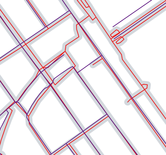
The following image shows the tool applied to a sample of OpenStreetMap (red) and official data published by the city of Vienna (purple) at Wien Handelskai. OSM was used as a reference graph and the buffer size was set to 10 meters.

In general, both graphs agree quite well. The percentage of the official graph within 10 meters of the OSM graph is 93% in the 20th district. In the above image, we can see that links available in OSM are not contained in the official graph (mostly pedestrian/bike links) and there seem to be some connectivity issues as well in the upper right corner of the image.

In my opinion, Processing models are a great solution to document geoprocessing work flows and share them with others. If you want to collaborate on building more models for OSM-related analysis, just leave a comment bellow.

Inspired by Václav Petráš posting about “Did you know that you can see streets of downtown Raleigh in elevation data from NC sample dataset?” I wanted to try the new GRASS GIS 7 Addon r.shaded.pca which creates shades from various directions and combines then into RGB composites just to see what happens when using the new EU-DEM at 25m.

To warm up, I registered the “normally” shaded DEM (previously generated with gdaldem) with r.external in a GRASS GIS 7 location (EPSG 3035, LAEA) and overlayed the OpenStreetMap layer using WMS with GRASS 7′s r.in.wms. An easy task thanks to University of Heidelberg’s www.osm-wms.de. Indeed, they offer a similar shading via WMS, however, in the screenshot below you see the new EU data being used for controlling the light on our own:

OpenStreetMap shaded with EU DEM 25m (click to enlarge)

Next item: trying r.shaded.pca… It supports multi-core calculation and the possibility to strengthen the effects through z-rescaling. In my example, I used:

r.shaded.pca input=eu_dem_25 output=eu_dem_25_shaded_pca nproc=3 zmult=50

The leads to a colorized hillshading map, again with the OSM data on top (50% transparency):

OpenStreetMap shaded with r.shaded.pca using EU DEM 25m (click to enlarge)

Yes, fun – I like it

Data sources:

• Shaded maps produced using Copernicus data and information funded by the European Union – EU-DEM layers
• © OpenStreetMap contributors

The post Using the 25m EU-DEM for shading OpenStreetMap layers appeared first on GFOSS Blog | GRASS GIS Courses.

We’re planning a couple of training classes for March:

• Introduction to QGIS
• Extending QGIS with Python

Each is a one day class and we plan to run them back to back. If you are local or just want to come to Alaska in March for some spring skiing, northern lights viewing, or to experience the equinox, please hop over to GeoApt and let us know so we can plan accordingly.

I’m very pleased to announce that Packt Publishing is organizing a giveaway contest for Learning QGIS 2.0. All you need to do is comment below the post and win a free copy of Learning QGIS 2.0. Read on for more details.

Amongst other topics, Learning QGIS 2.0 covers:

• Loading and visualizing vector and raster data
• Creating and editing spatial data and performing spatial analysis
• Designing great maps and printing them

How to Enter?

Simply post your expectations for this book in comments section below and you could be one of the lucky participants to win a copy.

DeadLine: The contest will close in 7 days on December, 12th 2013. Winners will be contacted by email, so be sure to use your real email address when you comment!

Please note: Winners residing in the USA and Europe will receive print copies. Others will be provided with eBook copies.

EU DEM 25m upper Garda Lake area with Riva del Garda and Arco (Italy). 3D view in wxNVIZ – GRASS GIS 7

The 25m European Digital Elevation Model (EU-DEM, Version 1) is a Digital Surface Model (DSM) representing the first surface as illuminated by the sensors:

EU DEM Rotaliana with Mezzocorona and S. Michele (Italy). Produced using Copernicus data and information funded by the European Union – EU-DEM layers.

Its elevations were captured at 1 arc second postings (2.78E-4 degrees). The tiles are provided at 25m resolution in EU-LAEA (EPSG. 3035) projection, temporal coverage: 2000, published in Oct 2013. It is a realisation of the Copernicus programme, managed by the European Commission, DG Enterprise and Industry. Metadata are provided here. According to their “Methodology” page it is a hybrid product based on SRTM and ASTER GDEM data fused by a weighted averaging approach and it has been generated as a contiguous dataset divided into 1 degree by 1 degree tiles, corresponding to the SRTM naming convention. In addition to the DEM data, a colour shaded relief image over Europe is provided.

From the metadata page: “The EU-DEM data are provided as is, i.e. without a formal validation yet. An independent statistical validation is scheduled as part of the GIO land monitoring service activities, and will be made available in the course of 2014.”

1. Data download

Note that the GeoTIFF files are of major size, up to 5 GB:

• Download GeoTIFF tiles by file name
• Download GeoTIFF tiles by map based selection

Hint for GRASS GIS users: instead of importing the data, you can use r.external to simply register the GeoTIFF file within a EU LAEA projected location.

The post EU-DEM: new Digital Surface Model at 25m appeared first on GFOSS Blog | GRASS GIS Courses.

A new feature coming up in QGIS 2.2 will be the ability to style the current active atlas feature with a different symbol. This also extends to styling other layers based on the current feature geometry. This post is a quick preview of the upcoming 2.2 feature.

When a layer has been enabled for Atlas in the composer two new variables will be created $atlasfeatureid and $atlasgeometry. This are static expression variables so once set they are available anywhere in QGIS. These two new static variables will now be set for each feature when printing using the Atlas feature. This also means we can access them in the rule and label expressions to do some pretty cool styled maps.

Once defined we can then create a rule using the rule based renderer to highlight the active layer. We do this by using the expression $id = $atlasfeatureid. Simply put "Does this feature ID match the current atlas one"

That's pretty cool. The current feature (ID 0) in this case is green and the rest is gray. You will also note another new feature in 2.2 which is the ELSE rule. This rule will run when none of the other rules on it's level have passed or evaluated to true. We can use this ELSE rule to just style everything else as gray.

Why don't we one up this a little and just label the current active one.

You could also use a CASE expression do the same thing CASE WHEN $id = $atlasfeatureid THEN "name" END. Take your pick on which one you like the most.

What if we wanted to just show other layers features that are within the area, maybe we want to style them different if they are within an area, or outside of that area. Lets take a look at styling a tree layer that is only within the current atlas geometry.

We have geometry functions in the expression engine so lets use those here on our street trees layer:

I have nested the rule so that we can style the trees differently based on status but only if they are within the active atlas feature.

Remember this is dynamic so there is going to be a performance hit if you try and run this type of expression on many features. The expressions will run once per feature per map redraw so just be aware of how expensive this can become.

When we render the output to files we get what was expected.

A new feature coming up in QGIS 2.2 will be the ability to style the current active atlas feature with a different symbol. This also extends to styling other layers based on the current feature geometry. This post is a quick preview of the upcoming 2.2 feature.

When a layer has been enabled for Atlas in the composer two new variables will be created $atlasfeatureid and $atlasgeometry. This are static expression variables so once set they are available anywhere in QGIS. These two new static variables will now be set for each feature when printing using the Atlas feature. This also means we can access them in the rule and label expressions to do some pretty cool styled maps.

Once defined we can then create a rule using the rule based renderer to highlight the active layer. We do this by using the expression $id = $atlasfeatureid. Simply put "Does this feature ID match the current atlas one"

That's pretty cool. The current feature (ID 0) in this case is green and the rest is gray. You will also note another new feature in 2.2 which is the ELSE rule. This rule will run when none of the other rules on it's level have passed or evaluated to true. We can use this ELSE rule to just style everything else as gray.

Why don't we one up this a little and just label the current active one.

You could also use a CASE expression do the same thing CASE WHEN $id = $atlasfeatureid THEN "name" END. Take your pick on which one you like the most.

What if we wanted to just show other layers features that are within the area, maybe we want to style them different if they are within an area, or outside of that area. Lets take a look at styling a tree layer that is only within the current atlas geometry.

We have geometry functions in the expression engine so lets use those here on our street trees layer:

I have nested the rule so that we can style the trees differently based on status but only if they are within the active atlas feature.

Remember this is dynamic so there is going to be a performance hit if you try and run this type of expression on many features. The expressions will run once per feature per map redraw so just be aware of how expensive this can become.

When we render the output to files we get what was expected.

A new feature coming up in QGIS 2.2 will be the ability to style the current active atlas feature with a different symbol. This also extends to styling other layers based on the current feature geometry. This post is a quick preview of the upcoming 2.2 feature.

When a layer has been enabled for Atlas in the composer two new variables will be created $atlasfeatureid and $atlasgeometry. This are static expression variables so once set they are available anywhere in QGIS. These two new static variables will now be set for each feature when printing using the Atlas feature. This also means we can access them in the rule and label expressions to do some pretty cool styled maps.

Once defined we can then create a rule using the rule based renderer to highlight the active layer. We do this by using the expression $id = $atlasfeatureid. Simply put "Does this feature ID match the current atlas one"

That's pretty cool. The current feature (ID 0) in this case is green and the rest is gray. You will also note another new feature in 2.2 which is the ELSE rule. This rule will run when none of the other rules on it's level have passed or evaluated to true. We can use this ELSE rule to just style everything else as gray.

Why don't we one up this a little and just label the current active one.

You could also use a CASE expression do the same thing CASE WHEN $id = $atlasfeatureid THEN "name" END. Take your pick on which one you like the most.

What if we wanted to just show other layers features that are within the area, maybe we want to style them different if they are within an area, or outside of that area. Lets take a look at styling a tree layer that is only within the current atlas geometry.

We have geometry functions in the expression engine so lets use those here on our street trees layer:

I have nested the rule so that we can style the trees differently based on status but only if they are within the active atlas feature.

Remember this is dynamic so there is going to be a performance hit if you try and run this type of expression on many features. The expressions will run once per feature per map redraw so just be aware of how expensive this can become.

When we render the output to files we get what was expected.

Processing has received a series of updates since the release of QGIS 2.0. (I’m currently running 2.0-20131120) One great addition I want to highlight today is the improved script editor and the help file editor.

Script editor

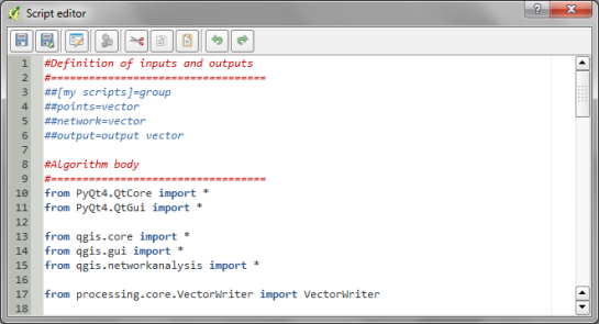
The improved script editor features a toolbar with commonly used tools such as undo and redo, cut, copy and paste, save and save as …, as well as very useful run algorithm and edit script help buttons. It also shows the script line numbers which makes it easier to work with while debugging code.

The model editor has a similar toolbar now which allows to export the model representation as an image, run the model or edit the model help.

Help editor

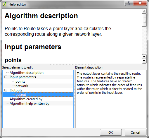
When you press the edit script help button, you get access to the new help editor. It’s easy to use: On the top, it displays the current content of the help file. On the bottom-left, it lists the different sections of the help file which can be filled with information. In the input parameters and outputs section, the help editor automatically lists the all parameters specified in the script code. Finally, in the bottom-right, you can enter the description. The resulting help file is saved in the same location as the original script under the name <scriptname>.py.help.