Related Plugins and Tags

QGIS Planet

(Fr) Oslandia recrute : ingénieur(e) développement C++ / Python – OSL2011B

Sorry, this entry is only available in French.

More icons & symbols for QGIS – updated

The 2016 post More icons & symbols for QGIS still regularly makes it to the top 10 list of posts by visitors. I wouldn’t attribute this popularity to the quality of this particular post, however. Instead, it’s a pretty clear sign that QGIS users are actively searching for more styling resources to add to their installations.

When it comes to styling resources, the person to follow right now is clearly Klas Karlsson who’s been keeping a steady stream of styling-related posts coming to Twitter:

Additionally, he’s the master-mind behind QGIS Hub, a – currently prototypical – platform for sharing styling resources and print layout templates:

If you are interested in sharing styling resources, head over there. Similarly, if you want to lend a hand developing QGIS Hub, get in touch!

Store and visualize your raster in the Cloud with COG and QGIS

We have recently been working for the French Space Agency ( CNES ) who needed to store and visualize satellite rasters in a cloud platform. They want to access the image raw data, with no transformation, in order to fullfill deep analysis like instrument calibration. Using classic cartographic server standard like WMS or TMS is not an option because those services transform datasets in already rendered tiles.

We chose to use a quite recent format managed by GDAL, the COG (Cloud Optimize Geotiff) and target OVH cloud platform for it provides OpenStack, a open source cloud computing platform.

How it works

A COG file is a GEOTiff file which inner structure is tiled, meaning that the whole picture is divided in fixed size tile (256 x 256 pixels for instance) so you can efficiently retrieve parts of the raster. In addition to the HTTP/1.1 standard feature range request, it is possible to get specific tiles of an image through the network without downloading the entire raster.

We used a service provided by OpenStack, called Object Storage to serve the COG imagery. Object storage allows to store and retrieve file as objects using HTTP GET/POST requests.

Why not WCS ?

Web Coverage Service standard could have been an option. A WCS server can serve raw data according to a given geographic extent. It’s completely possible to deploy a container or a VPS (Virtual Private Server) running a WCS Server in a cloud plateform. The main advantages of the COG solution over WCS Server is that you don’t have to deal with the burden of deploying a server, like giving it ressources, configuring load balancing, handle updates, etc…

The beauty of COG solution is its simplicity. It is only HTTP requests, and everything else (rendering for instance) is done on the client side.

Step by step

Here are the different steps you’d have to go through if you’re willing to navigate in a big raster image directly from the cloud.

First, let’s generate a COG file

gdal_translate inputfile.tif cogfile.tif -co TILED=YES -co COPY_SRC_OVERVIEWS=YES -co COMPRESS=DEFLATE

Install your openstack-client, it can be achieved easily with Python pip install command line

$ pip install python-openstackclient

Next, configure your openstack client in order to generate an athentification token. To do so you need to download your project specific openrc file to setup your environment)

$ source myproject-openrc.sh
Please enter your OpenStack Password for project myproject as user myuser:
**********
$ openstack token issue                                 
+------------+-----------------------------------------------------------------------------------------------------------------------------------------------------------------------------------------+
| Field      | Value                                                                                                                                                                                   |
+------------+-----------------------------------------------------------------------------------------------------------------------------------------------------------------------------------------+
| expires    | 2020-07-21T08:15:12+0000                                                                                                                                                                |
| id         | xxxx_my_token_xxxx
| project_id | 97e2e750f1904b41b76f80a50dabde0a                                                                                                                                                        |
| user_id    | 18f7ccaf1a2d4344a4e35f0d84eb065e                                                                                                                                                        |
+------------+-----------------------------------------------------------------------------------------------------------------------------------------------------------------------------------------+

You are now good to push you COG file to the cloud instance

openstack object create MyContainer cogfile.tif --name cogfile.tif

Before starting QGIS, 2 environment variables need to be set.  (replace xxxx_my_token_xxxx with the token you’d just come to generate)

$ export SWIFT_AUTH_TOKEN=xxxx_my_token_xxxx
$ export SWIFT_STORAGE_URL=https://storage.sbg.cloud.ovh.net/v1/AUTH_$OS_PROJECT_ID

It can also be done directly from the QGIS Python console by setting those variable using the os.environ.

Finally, add a cloud raster data source in in QGIS

You can now navigating into your image directly reading it from the cloud

© CNES 2018, Distribution Airbus DS

Performances

While panning in the map, QGIS will download only few tiles from the image in order to cover the view extent. The display latency that you could see in the video depends essentially on:

  • The number of band of your image
  • The pixel size
  • Your internet connection (mine, the one use for the video, is not an awesome one)

Note that the white flickering that you could see when you move in the map and the raster is refreshed should be removed in next version of QGIS according to this QEP.

What’s next ?

Thanks so much to the GDAL and QGIS contributors for adding such a nice feature ! It brings lots of possibilities for organizations that have to deal with great number of big raster and just want to explore part of it.

We are already thinking about further improvments (ease authentification, better integration with processing…), so if you’re willing to fund them or just want to know more about QGIS, feel free to contact us at [email protected]. And please have a look at our support offering for QGIS.

Line Label Placement: Our gift to the QGIS community!

If you’re a follower of North Road’s social media accounts, it probably comes as no surprise to hear that we love sharing regular tips and useful suggestions about working with spatial data on these channels. Recently, we realised we were close to a new milestone of 4k followers of our Twitter stream. This milestone gave us the perfect excuse to give something back to all these followers! So we ran a little promo, where we promised that if we hit 4k followers we’d implement a new feature in QGIS, as determined by a popular vote:

Given we’ve now reached the target milestone, it was our turn to deliver! So we’re proud to introduce a new feature coming in QGIS 3.16: the ability to control exactly where labels are positioned along line feature! Let’s take a look!…

In previous QGIS releases, whenever labels are enabled for a line layer these labels will automatically gravitate towards the center of the line features:

In certain situations, it’s desirable for these labels to be positioned in specific positions along these line features (e.g. at the start of lines, or at the end of lines). With this new feature gift to the community, QGIS users have to option to precisely control the label placement for these lines:


There’s new options for placing the labels at the start of lines, end of lines, or at a custom offset along the line.

This option can be super-handy when combined with Rule Based Labelling, as it allows you to have different labels at the start versus end of lines:

So there we go! Another great QGIS cartography enhancement, heading your way in QGIS 3.16, and just a little thank you back to the community for all your support of North Road.

And if you’re not following us on social media yet, it’s a great to start… because who knows when our next little giveaway will be?!


Publication de l’extension COVADIS RAPEA pour QWAT et QGEP

QWAT est une application open source de gestion des réseaux d’eau potable émanant des collectivités de Pully, le SIGE à Vevey, Morges et Lausanne.
QGEP est son homologue dédiée à la gestion des eaux usées et pluviales, initiée par le groupe utilisateur QGIS Suisse.

L’échange de données entre institutions est une pierre angulaire des politiques de l’eau. Ces échanges se basent sur des formats d’échanges standardisés. Ainsi les Cantons de Fribourg (format aquaFRI) ou de Vaud (format SIRE) conditionnent certaines subventions publiques à la transmission des données selon des formats pré-définis et permettent à ces échelons administratifs d’avoir une vision globale des réseaux humides.

Dans le cadre d’une expérimentation des outils QWAT (eau potable) et QGEP (eaux usées), Charentes Eaux a souhaité mettre en œuvre des extensions dédiées au standard d’échange de données sur les réseaux d’eau Français, le Géostandard Réseaux d’adduction d’eau potable et d’assainissement (RAEPA) défini par la Commission de validation des données pour l’information spatialisée (COVADIS).

Oslandia a été mandaté pour mettre en œuvre des instances de QWAT et QGEP, réaliser les extensions RAEPA pour chacun de ces outils, et aider Charente Eaux à charger les données des collectivités membres de ce syndicat mixte.

https://charente-eaux.fr/le-syndicat/qui-sommes-nous/

Le travail a été publié pour QWAT sous forme d’une extension standardisée dans le dépôt l’organisation QWAT https://github.com/qwat/extension_fr_raepa/

Pour QGEP, il n’existe pas encore de fonctionnalité pour gérer d’extension, le dépôt https://gitlab.com/Oslandia/qgep_extension_raepa/ contient donc les définitions de données et de vues à rajouter manuellement au modèle de données.

La compatibilité des modèles de données a été évaluée et le choix a été fait de ne faire que des vues dédiées à l’export de données. Il est techniquement possible de faire des vues éditables pour permettre le chargement de données via ces vues depuis des fichiers suivant le gabarit de données RAEPA. Le niveau de simplification et d’agrégation des listes de valeurs rend ce travail peu générique dans l’état actuel du géostandard (v1.1), il est donc plus pertinent à ce stade de réaliser des scripts de chargement sans passer par ce pivot dans le cas de Charente-Eaux

Announcing the Point Cloud Data in QGIS Crowdfunding Campaign!

With the recent advancements in LiDAR survey technology and photogrammetry there has been a huge demand in capturing and storing point cloud data. Point cloud data are vector in nature, but are usually orders of magnitude larger than a standard vector layer. Typical vector datasets range from thousands to millions of features, while point clouds range from millions to billions or even trillions of points. Due to this sheer number of points a completely different approach to visualise, analyse and store point clouds is needed in a GIS platform.

Integrating a point cloud viewer in a desktop GIS application adds a lot of value for users compared to a specialised and dedicated point cloud viewer:

  • Point cloud data can be visualised, compared, and analysed alongside other types of spatial data (including vector, raster and mesh layers)
  • A familiar user interface and workflows
  • Integration with analytical tools to quickly create derived datasets

Despite these benefits, current versions of the QGIS desktop application do not support visualisation of point cloud data. With our partners at Lutra Consulting and Hobu, we have decided to bridge this missing gap and add point cloud support in QGIS, and are launching a new crowdfunding campaign to fund this work!

Head on over to the official crowd funding page here for the full details of the campaign, and for details on how you can contribute and make this work a reality.

Announcing SLYR Community Edition

North Road are proud to announce the official release of SLYR Community Edition, a new open-source version of our powerful SLYR ESRI to Open Source compatibility suite. The Community Edition is available for download from the official QGIS plugin repository today, for QGIS versions 3.4 and above. It supports automated conversion of ESRI .style symbol databases, including conversion of markers, fills, line styles and color ramps to their closest QGIS symbology equivalent, allowing users to instantly transition their style libraries into QGIS!

If you’ve followed our work in the past, it will come as no surprise to hear that North Road are passionate about open source geospatial, and for reducing the barriers which users encounter when moving to open-source software. We see our SLYR tool as an integral part of this process, and the licensed version of the plugin currently supports automated conversion of MXD, LYR, PMF, and other ESRI-specific formats to QGIS documents.

Our intention all along has been to make this tool freely available for all users of open-source geospatial software, and to release our work under a permissive, open-source license so that other projects can take advantage of our reverse engineering efforts. That’s why we made an “open source pledge” a fundamental part of our SLYR tool development! By the terms of this pledge, exactly six months after we hit staged preset funding levels we will open-source more components of the code and update the community version of the plugin accordingly. (This approach gives motivated organisations instant access to the full functionality of the SLYR tool via a license purchase, or free access to a subset of this functionality via the community edition of the plugin. It allows us to heavily invest in further reverse-engineering efforts and improvements to the plugin, to QGIS, and to the wider open-source geospatial community.)

If you’re keen to explore transitioning your workplace from ESRI to open-source, send us an email to discuss what we can offer! North Road staff have years of experience in implementing open-source geospatial solutions within commercial workplaces, and for setting up dual commercial-and-open-source friendly environments.

QField 1.4 released – Happy new year

What a year’s start! After a very packed December publishing all the QGIS on the road videos and quietly releasing QField 1.3 – Ben Nevis we could have gone and relaxed over the holidays. But since we love QField so much we immediately started working on the next iteration. Now, after an intensive testing period, we are proud to announce the release of QField 1.4 – Olavtoppen.

Olavtoppen!? yes, the highest point of Bouvet Island, the remotest island on Earth. And sure enough, QField would follow you there!

As usual, get it on play store or download it from GitHub.

QField Crowdfunding Campaign

Before digging into all the new goodness that you will find in QField 1.4, let’s get a big “Thanks” out to everybody who supported our crowdfunding campaign for improved camera support and all our customers that agreed to open source the work we did for them.

If you like QField, want a new feature or would like to support the project, don’t hesitate to get in touch with us.

Usability enhancements

In QField 1.2 we started to improve on the usability of the user interface. We are constantly working on this with a usability expert to get the user interface to be even more appealing and user-friendly.

Besides lots of clean-up and polishing, QField received two major improvements, a portrait mode and a new welcome screen with recent projects.

Welcome screen with recent projects

QField is all about efficiency. While favourites folders in the file selector already give a great productivity boost, very often we work with the same 3-4 projects. This is why we redesigned the welcome screen to list the last five project used. And if you look carefully you might get a hint of what will be coming soon…

Portrait mode

QField now flawlessly works in portrait mode. We heard you say you needed a comfortable way to work in portrait mode, especially on smartphones. QField forms and button placements are now optimized to be easy to use with your thumbs.

New features

We keep on listening to your feedback and prioritize new features based on it. We did implement some minor features like allowing hiding legend nodes and printing to PDF using the current extent. But this time’s superstars are three highly expected features: Splitting of geometries, compass integration and, yes you guessed right, native camera and gallery app support!

Split Features

ezgif com-optimize

A new editing tool is available that allows for splitting existing features. This adds an even more powerful operation to an already impressive geometry editing tools set.

Compass integration

A long-awaited feature! QField now shows you on-screen in which direction you are looking, walking, driving, flying or warping direction. This makes it much easier and more pleasant to navigate in the field.

Screenshot_20200115-154223_QField Nightly

Native Camera and Gallery

It is now possible to use your favourite camera app so that you have more control over how pictures are taken. It is also possible to select pictures which are already on your device by using the new gallery selector.

Pro Tip: You can use any camera app. For example, you can use the open camera app to create geotagged photos if your preinstalled system camera doesn’t save positioning information in EXIF data.

Pro Tip 2: You can use an image annotation app to add notes, sketches, drawings and so on to your images and then choose them from QField via the add from gallery button.

Antenna Height Correction

For high precision measurements, it’s possible to compensate your altitude by a fixed antenna height. This will then automatically adjust all the digitised altitude values.

JPEG 2000

Support for JPEG 2000 raster datasets was added. This lossy format offers a compression rate at par with proprietary formats like ECW or Mr SID.

Pro Tip: save your base maps in JPEG 2000 to save storage.

New Languages

Thanks to the hard work of our community, QField is now also available in Turkish and Japanese.

New packages

You say: wow that’s a lot! We say: there is more 🙂
We have upgraded our whole building infrastructure so that you can comfortably get even more QField goodness without having to uninstall your production ready QField.

Automated master builds

After each pull request is merged into our master code, a new package is created and automatically published on the playstore in a dedicated app called QField for QGIS – Unstable (Early Access). Installing this app will allow you to always have the latest build of QField for testing and giving feedback. On your device, this app is completely separated from the production-ready QField and has a distinctive black icon so that you do not confuse it.

Pull request builds

QField is an extremely active project, and as you see we develop multiple functionalities and fixes at the same time. If you’re particularly interested in one of this, our continuous integration fairy builds and publishes new packages automatically at each commit directly to the pull request you are interested in. To see what we are currently working on, have a look at the pull request overview page.

Experimental Windows builds

Last but definitely not least, we’ve set up an Azure CI infrastructure to build QField for windows. For now, we still consider this experimental but we already had some very successful testing. If you are interested in testing out QField for windows you can get it here, remember it is experimental so don’t use it in production yet and give us as much feedback as possible 🙂

What’s next?

As you can imagine we’ve had a very busy start of 2020, but even more is to come soon with the next releases of QField. We’d like to thank again all companies and individuals that actively use QField and that invest in making QField even better. If you feel QField misses something you need or would like to support the project, don’t hesitate to get in touch with us.

Offline WMS – Benchmarking raster formats for QField

What are we looking for?

We would like to use WMS offline on QField. For that, we need to figure out what is the best way to get a raster from a WMS and which format is the most efficient (size and performance).

In this post we’ll show you is how to generate the ideal raster file from a WMS and the results of our efficiency tests for the the different raster formats.

WMS to GPKG

The simple way

If there is no limitation on the WMS or you need only a small region, here is the easiest process.

  1. Request the WMS and store a description file in XML:
gdal_translate "WMS:url" file.xml -of WMS
  1. Create a Geopackage from the information in the description file.
gdal_translate -of GPKG file.xml file.gpkg -co TILE_FORMAT=JPEG

That was quite simple, right?

The larger datasets way

If the command takes too much time, it means that it is trying to download too much data and could be caused by downloading higher resolution data than required.
The command might even completely fail if it contains a request for bigger data blocks thant the server allows.

Here is the process to get larger datasets in a simple way. Let’s use a real example:

  1. Use gdal_translate "WMS:https://www.gebco.net/data_and_products/gebco_web_services/web_map_service/mapserv?request=getmap&service=wms&crs=EPSG:4326&format=image/jpeg&layers=gebco_latest&version=1.1.0" test.xml -of WMS
  2. Open the test.xml file for editing, here you’ll find the parameters of the WMS. We change the “SizeX” to 3600 and “SizeY” to 1800. By changing these parameters we lower the resolution. It is important to keep proportionality.
  3. Another thing we need to change are “BlockSizeX” and “BlockSizeY” that define the size of the tiles. We change both to 2048.
  4. Finally, use gdal_translate -of GPKG test.xml test.gpkg -co TILE_FORMAT=JPEG
  5. To make a Geopackage pyramid use gdaladdo GPKG:test.gpkg:gebco_latest. It will replace the Geopackage, if you want to keep the original one, you need to copy it first.

Now you have a raster Geopackage that you can use in QField.

Testing raster formats

Preparing the files

As first step we exported our test orthophoto WMS to a plain GeoTIFF using QGIS’ default behaviour.

Default parameters used to create the initial tiff
Formatgdal_translategdaladdo
gpkg JPEGgdal_translate -of GPKG “C:\test\ortho_test.tif” “C:\test\test_JPEG.gpkg” -co TILE_FORMAT=JPEG
gpkg PNGgdal_translate -of GPKG “C:\test\ortho_test.tif” “C:\test\test_PNG.gpkg” -co TILE_FORMAT=PNG
gpkg PNG_JPEGgdal_translate -of GPKG “C:\test\ortho_test.tif” “C:\test\test_PNG_JPEG.gpkg” -co TILE_FORMAT=PNG_JPEG
gpkg PNG8gdal_translate -of GPKG “C:\test\ortho_test.tif” “C:\test\test_PNG8.gpkg” -co TILE_FORMAT=PNG8
gpkg WEBPgdal_translate -of GPKG “C:\test\ortho_test.tif” “C:\test\test_WEBP.gpkg” -co TILE_FORMAT=WEBP
gpkg pyramid_JPEGgdal_translate -of GPKG “C:\test\ortho_test.tif” “C:\test\test_JPEG.gpkg” -co TILE_FORMAT=JPEGgdaladdo GPKG:C:\test\test_JPEG.gpkg:test_gpkg_JPEG
gpkg pyramid_PNGgdal_translate -of GPKG “C:\test\ortho_test.tif” “C:\test\test_PNG.gpkg” -co TILE_FORMAT=PNGgdaladdo GPKG:C:\test\test_PNG.gpkg:test_gpkg_PNG
gpkg pyramid_PNG_JPEGgdal_translate -of GPKG “C:\test\ortho_test.tif” “C:\test\test_PNG_JPEG.gpkg” -co TILE_FORMAT=PNG_JPEGgdaladdo GPKG:C:\test\test_PNG_JPEG.gpkg:test_gpkg_PNG_JPEG
gpkg pyramid_PNG8gdal_translate -of GPKG “C:\test\ortho_test.tif” “C:\test\test_PNG8.gpkg” -co TILE_FORMAT=PNG8gdaladdo GPKG:C:\test\test_PNG8.gpkg:test_gpkg_PNG8
gpkg pyramid_WEBPgdal_translate -of GPKG “C:\test\ortho_test.tif” “C:\test\test_WEBP.gpkg” -co TILE_FORMAT=WEBPgdaladdo GPKG:C:\test\test_WEBP.gpkg:test_gpkg_WEBP
JPEG2000gdal_translate -of JP2OpenJPEG “C:\test\ortho_test.tif” “C:\test\test_jpeg_2000.jpg”
COG DEFLATEgdal_translate “C:\test\ortho_test.tif” “C:\test\test_cog.tif” -co TILED=YES -co COPY_SRC_OVERVIEWS=YES -co COMPRESS=DEFLATE
COG_JPEGgdal_translate “C:\test\ortho_test.tif” “C:\test\test_cog_JPEG.tif” -co TILED=YES -co COPY_SRC_OVERVIEWS=YES -co COMPRESS=JPEG
tifIn QGIS right click on the layer > export > save as > (see the details in the picture under the table)
MBTgdal_translate -of MBTILES “C:\test\ortho_test.tif” “C:\test\test_mbt.mbtiles”
Creation commands for all the tested formats

Rendering test results

We have tested many formats, here is a table with the results of the size and rendering speed in QGIS and QField.
To analyze the speed we used qgis_bench.exe -i 10 -p "C:\test\test.qgs" >> "C:\test\test.log.
Qgis_bench is a tool that renders a QGIS project a number of times to get performance measurements. The parameter -i is to define the iterations and -p is the project used which contains only the generated raster.

FormatExtent [m]File size [GB]Total_avgTotal_maxdevTotal_minTotal_stdev
gpkg JPEG52’880/29’2300.4250.242255.7815.539244.984
gpkg PNG52’880/29’2302.9412.002490.328152.142259.859
gpkg PNG_JPEG52’880/29’2300.4250.125256.8756.750245.172
gpkg PNG852’880/29’2301.4283.875296.40612.625271.250
gpkg WEBP52’880/29’2300.3330.238348.10973.534256.703
gpkg pyramid_JPEG52’880/29’2300.51.0093.4062.3970.688
gpkg pyramid_PNG52’880/29’2303.01.2083.2812.0730.688
gpkg pyramid_PNG_JPEG52’880/29’2300.61.4914.3442.8531.016
gpkg pyramid_PNG852’880/29’2301.61.5084.3752.8670.969
gpkg pyramid_WEBP52’880/29’2300.41.3334.9063.5730.766
JPEG200052’880/29’2301.113.888136.109122.2220.219
COG DEFLATE52’880/29’2303.6264.427273.09425.411239.016
COG_JPEG52’880/29’2301.014.778131.172116.3941.734
tif52’880/29’2306.42.3676.7344.3671.672
MBT52’880/29’2304.40.4694.6414.1710
Comparison of file size and rendering speed of different raster formats. “Total” columns are rendering times in [s]. Lower file size is more storage friendly, lower Total_avg is more performant.

Analysis

File size

The Geopackage WEBP (with and without pyramid) has the best result for file size, but it is not yet supported by QField (from 1.6) and is only slightly smaller than the JPEG variant.

Plain GeoTiff, MBTiles, Cloud Optimized GeoTIFF (COG – DEFLATE mode) and Geopackages with PNG generate by far the largest file sizes (up to 20x larger) and are thus not recommended.

Rendering speed

MBTiles are on average double as fast as JPEG Geopackages with pyramids which in turn are more than double as fast as GeoTIFF and 15x faster than COG.
Geopackages without pyramids are 200 to 400 times slower.

Conclusion

Even though MBTiles render faster than the Geopackage pyramid JPEG, they come with an almost 10x bigger storage requirement which makes us say that the best offline raster format supported by QField is Geopackage pyramid JPEG or if you need transparency and slightly smaller files Geopackage pyramid WebP.

If you need transparency before QField 1.6, the best results are achieved with Geopackage pyramid PNG_JPEG.

Marco becomes QGIS.org Chair

Serving as a pragmatic community conciliator – collecting thoughts from people with differing opinions and trying to find the high road through difficult issues – I want to focus my and the community’s energies on our core product, QGIS.

Marco Bernasocchi · QGIS.org Chair

OPENGIS.ch has always been dedicated to sustaining QGIS’ technological and economical well-being, supporting it with endless hours of internally funded QA, infrastructure works and developments.

Today we are very proud to announce that our commitment has grown even more as one of our founders and CEO Marco Bernasocchi was elected Chair of the QGIS.org association.

With over 15 years of involvement with QGIS (he started working with QGIS 0.6) and two years serving as vice-chair, Marco will serve for the next two years as Chairperson of the QGIS.org association.

Understanding the importance of the role trusted him, Marco would like to thank the QGIS community for the trust and appreciation. Marco is looking forward to intensifying work with the PSC and the fantastic QGIS community to push QGIS even further.

We wish Marco and the rest of the elected PSC two very successful years full of QGIS awesomeness.

Rock on QGIS! – read more at QGIS Annual General Meeting – 2020

Marco’s vision for QGIS.org:

I want to help QGIS and it’s community thrive under the value proposition of:

Making the most amazing opensource GIS that provides users with value and that meets their needs by providing great functionality and usability, being cost-effective whilst being actively supported by a vibrant and knowledgeable community.

Sharing our work under an open-source license is part of the approach by which we achieve that value proposition as it allows broad collaboration with our developers and users community.

I see FOSS as a very socially responsible way to develop software, but even more, I see the immense technological advantage that writing open-source code brings. This is why I want our focus to be on allowing both pragmatic and ideological views to respectfully coexist and enrich each other.

One of my main motivations to be part of the PSC and to make myself available as project Chair is to help QGIS keep this incredible growth rate by being even more attractive to new community members, sponsors and large/corporate users. To achieve this, the key is maintaining the right balance between sustainable processes (that guarantee the great quality QGIS has been known for) and an interesting and motivating grassroots project to ensure that QGIS remains an attractive project for volunteers to contribute to and help QGIS and its community to grow to become even more the reference [Open Source] GIS project.

Plugin Manager improvement

During the 2020 Swiss QGIS Users Group annual meeting, a proposal to improve the plugin manager was accepted to improve QGIS’ plugin manager. Starting with version 3.14, it will be possible to choose whether to install the stable or the experimental version of individual plugins.

This feature will greatly improve the workflow between developers and users of a plugin. Users will be able to easily switch between the stable version used in production, and the experimental version to test out new features.

Until now, it was necessary either to configure a dedicated extensions repository or to have users manually install development version from a zip file.

You can test out this new feature before 3.14 is out by installing a recent nightly build of QGIS and making sure you have enabled the “show experimental versions” in the plugin manager.

We’re very thankful to the Swiss QGIS User Group for funding this new feature!

Versie 3.5.0 van de PDOKServicesPlugin

OK, this is a short post to let the dutchies know there is a new version 3.5.0 of the PDOKServicesPlugin to load some of our national data as WMS, WFS or WCS. For example: the GeoMorphological map of The Netherlands, or the data of the accidents that happened from 2008 till 2018. Here combined in […]

(Fr) Financement mutualisé du logiciel libre: le cas QGIS

Sorry, this entry is only available in French.

Securely accessing enterprise ArcGIS Portal sites through QGIS

An updated version of this guide is available!

We were recently contacted for advice regarding our recommendations for securely accessing content on an enterprise ArcGIS Portal deployment from within QGIS. Fortunately, this setup is fully supported and works seamlessly in QGIS, thanks to the native integration of “OAuth2” authentication in QGIS!

This post details step-by-step instructions in setting up both ArcGIS Portal and QGIS to enable this integration. First, we’ll create a new desktop application on the Portal site in order to obtain the application-specific access keys for OAuth2 authentication. We’ll then create an authentication configuration in QGIS and associate this with a connection to the Portal site. Let’s dive in by doing the Portal configuration first…

Creating an application

Logon to the Portal, and from the “Content” tab, click the “Add Item” option. Select “An application” from the drop down list of options:

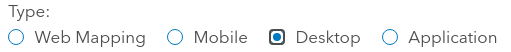
Set the type of the application as “Desktop

You can fill out the rest of this dialog as you see fit. Suggested values are:

  • Purpose: Ready to Use
  • Platform: Qt
  • URL: http://qgis.org
  • Tags: QGIS, Desktop, etc

Now – here comes a trick. Portal will force you to attach a file for the application. It doesn’t matter what you attach here, so long as it’s a zip file. While you could attach a zipped copy of the QGIS installer, that’s rather wasteful of server space! We’d generally just opt for a zip file containing a text file with a download link in it.

Click Add Item when you’re all done filling out the form, and the new application should be created on the Portal.

Registering the Application

The next step is to register the application on Portal, so that you can obtain the keys required for the OAuth2 logon using it. From the newly created item’s page, click on the “Settings” tab:

Scroll right to the bottom of this page, and you should see a “Register” button. Press this. Set the “App type” to “Native“.

Add two redirect URIs to the list (don’t forget to click “Add” after entering each!):

  1. The Portal’s public address, e.g. https://mydomain.com/portal
  2. http://127.0.0.1:7070

Finally, press the “Register” button in the dialog. If all goes well then the App Registration section in the item settings should now be populated with details. From here, copy the “App ID” and “Secret” strings, we’ll need these later:

Determine Request URLs

One last configuration setting we’ll need to determine before we fire up QGIS is the Portal’s OAuth Request and Token URLs. These are usually found by appending /sharing/rest/oauth2/authorize and /sharing/rest/oauth2/token to the end of your Portal’s URL.

For instance, if your public Portal URL is http://mydomain.com/portal, then the URLs will be:

Request URL: http://mydomain.com/portal/sharing/rest/oauth2/authorize
Token URL: http://mydomain.com/portal/sharing/rest/oauth2/token

You should be able to open both URLs directly in a browser. The Request URL will likely give a “redirect URL not specified” error, and the Token URL will give a “client_id not specified” error. That’s ok — it’s enough to verify that the URLs are correct.

We’re all done on the Portal side now, so time to fire up QGIS!

Creating an QGIS OAuth2 Authentication Configuration

From your QGIS application, select Options from the Settings menu. Select the Authentication tab. We need to create a new authentication configuration, so press the green + button on the right hand side of the dialog. You’ll get a new dialog prompting you for Authentication details.

There’s a few tricks to this setup. Firstly, it’s important to ensure that you use the exact same settings on all your client machines. This includes the authentication ID field, which defaults to an auto-generated random string. (While it’s possible to automatically deploy the configuration as part of a startup or QGIS setup script, we won’t be covering that here!).

So, from the top of the dialog, we’ll fill in the “Name” field with a descriptive name of the Portal site. You then need to “unlock” the “Id” field by clicking the little padlock icon, and then you’ll be able to enter a standard ID to identify the Portal. The Id field is very strict, and will only accept a 7 letter string!

Drop down the Authentication Type combo box, and select “OAuth2 Authentication” from the list of options. There’s lots of settings we need to fill in here, but here’s what you’ll need:

  • Grant flow: set to “Authorization Code”
  • Request URL: enter the Request URL we determined in the previous step, e.g. http://mydomain.com/portal/sharing/rest/oauth2/authorize
  • Token URL: enter the Token URL from the previous step, e.g. http://mydomain.com/portal/sharing/rest/oauth2/token
  • Refresh Token URL: leave empty
  • Redirect URL: leave as the default http://127.0.0.1:7070 value
  • Client ID: enter the App ID from the Portal item’s App Registration information (see earlier steps)
  • Client Secret: enter the App Secret from the Portal item’s App Registration information (see earlier steps)
  • Scope: leave empty
  • API Key: leave empty

That’s it — leave all the rest of the settings at their default values, and click Save.

You can close down the Options dialog now.

Adding the Portal Connection Details

Lastly, we’ll need to setup the Portal connection as an “ArcGISFeatureServer” and “ArcGISMapServer” connection in QGIS. This is done through the QGIS “Data Source Manager” dialog, accessed through the Layer menu. Click the “ArcGIS Feature Server” tab to start with, and then press “New” in the Server Connections group at the top of this dialog.

Enter a descriptive name for the connection, and then enter the URL for the ArcGIS server REST endpoint associated with your Portal:

Lastly, select the new OAuth2 configuration you just created under the “Authentication” group:

Click OK, and you’re done! When you try to connect to the newly added connection, you’ll automatically be taken to the Portal’s logon screen in order to authenticate with the server. After entering your details, you’ll then be connected securely to the server and will have access to all items which are shared with your user account on the Portal!

You can then repeat this step for and create a similar connection under the “ArcGIS Map Server” tab.

We’ve regularly use this setup for our enterprise clients, and have found it to work flawlessly in recent QGIS versions! If you’ve found this useful and are interested in other “best-practice” recommendations for mixed Open-Source and ESRI workplaces, don’t hesitate to contact us to discuss your requirements… at North Road we specialise in ensuring flawless integration between ESRI based systems and the Open Source geospatial software stack.
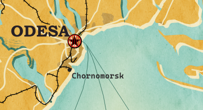
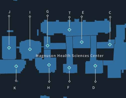
Movement data in GIS #30: synchronized trajectory animations with QGIS temporal controller

QGIS Temporal Controller is a powerful successor of TimeManager. Temporal Controller is a new core feature of the current development version and will be shipped with the 3.14 release. This post demonstrates two key advantages of this new temporal support:

  1. Expression support for defining start and end timestamps
  2. Integration into the PyQGIS API

These features come in very handy in many use cases. For example, they make it much easier to create animations from folders full of GPS tracks since the files can now be loaded and configured automatically:

Script & Temporal Controller in action (click for full resolution)

All tracks start at the same location but at different times. (Kudos for Andrew Fletcher for recordings these tracks and sharing them with me!) To create an animation that shows all tracks start simultaneously, we need to synchronize them. This synchronization can be achieved on-the-fly by subtracting the start time from all track timestamps using an expression:

directory = "E:/Google Drive/QGIS_Course/05_TimeManager/Example_Dayrides/"

def load_and_configure(filename):
    path = os.path.join(directory, filename)
    uri = 'file:///' + path + "?type=csv&escape=&useHeader=No&detectTypes=yes"
    uri = uri + "&crs=EPSG:4326&xField=field_3&yField=field_2"
    vlayer = QgsVectorLayer(uri, filename, "delimitedtext")
    QgsProject.instance().addMapLayer(vlayer)

    mode = QgsVectorLayerTemporalProperties.ModeFeatureDateTimeStartAndEndFromExpressions
    expression = """to_datetime(field_1) -
    make_interval(seconds:=minimum(epoch(to_datetime("field_1")))/1000)
    """

    tprops = vlayer.temporalProperties()
    tprops.setStartExpression(expression)
    tprops.setEndExpression(expression) # optional
    tprops.setMode(mode)
    tprops.setIsActive(True)

for filename in os.listdir(directory):
    if filename.endswith(".csv"):
        load_and_configure(filename)

The above script loads all CSV files from the given directory (field_1 is the timestamp, field_2 is y, and field_3 is x), enables sets the start and end expression as well as the corresponding temporal control mode and finally activates temporal rendering. The resulting config can be verified in the layer properties dialog:

To adapt this script to other datasets, it’s sufficient to change the file directory and revisit the layer uri definition as well as the field names referenced in the expression.


This post is part of a series. Read more about movement data in GIS.

TimeManager is dead, long live the Temporal Controller!

TimeManager turns 10 this year. The code base has made the transition from QGIS 1.x to 2.x and now 3.x and it would be wrong to say that it doesn’t show ;-)

Now, it looks like the days of TimeManager are numbered. Four days ago, Nyall Dawson has added native temporal support for vector layers to QGIS. This is part of a larger effort of adding time support for rasters, meshes, and now also vectors.

The new Temporal Controller panel looks similar to TimeManager. Layers are configured through the new Temporal tab in Layer Properties. The temporal dimension can be used in expressions to create fancy time-dependent styles:

temporal1

TimeManager Geolife demo converted to Temporal Controller (click for full resolution)

Obviously, this feature is brand new and will require polishing. Known issues listed by Nyall include limitations of supported time fields (only fields with datetime type are supported right now, strings cannot be used) and worse performance than TimeManager since features are filtered in QGIS rather than in the backend.

If you want to give the new Temporal Controller a try, you need to install the current development version, e.g. qgis-dev in OSGeo4W.


Update from May 16:

Many of the limitations above have already been addressed.

Last night, Nyall has recorded a one hour tutorial on this new feature, enjoy:

QGIS video tutorials: election maps, hydrology, and more

Mapping spatial decision patterns, such as election results, is always a hot topic. That’s why we decided to include a recipe for election maps in our QGIS Map Design books. What’s new is that this recipe is now available as a free video tutorial recorded by Oliver Burdekin:

This video is just one of many recently published video tutorials that have been created by QGIS community members.

For example, Hans van der Kwast and Kurt Menke have recorded a 7-part series on QGIS for Hydrological Applications:

and Klas Karlsson’s Youtube channel is also always worth a follow:

For the Pythonically inclined among you, there is also a new version of Python in QGIS on the Automating GIS-processes channel:


(Fr) Entretien avec Vincent Picavet

Sorry, this entry is only available in French.

SLYR ESRI to QGIS compatibility suite – April 2020 update

Since the last update, our “SLYR” ESRI to QGIS compatibility suite has gained a ton of new functionality, including full support for conversion of ArcMap MXD documents (with page layouts!). In this update, we’ll explore some of the new functionality available in the tool — but instead of focusing solely on SLYR, this time we’ll also explore the enhancements we’ve been making in QGIS itself that have helped improve the quality of ArcMap document conversion.

While many of these enhancements are already available to all users of QGIS 3.12, others are exciting additions to the upcoming QGIS 3.14 release. Let’s dive in!

Improved legend customisation

One shortcoming we realised early on during our work on SLYR was that QGIS map legends just didn’t offer a comparable level of customisation as ArcMap legends. We could convert the basic layout of a legend, but we just couldn’t get the legend appearance in QGIS sufficiently close to its original appearance in the MXD file.

To address this we’ve been extending QGIS’ inbuilt legend support by adding finer control over the legend layout and spacing.

As a result, one exciting addition we’ve recently made for QGIS 3.14 is adding the ability to customise legend patch shapes and sizes on an item-by-item basis! Previously, legends in QGIS were rather boring, with all polygon layers showing as a plain rectangle and line layers as a horizontal line.

Now, users have full control over setting custom shapes for their legend patches! This makes for much more user-friendly legends, as you can now show representative shapes in your legends — e.g. a river symbol can be shown as a wiggly line, instead of an unrealistic straight horizontal line.

You can also override the size of a legend patch on an item-by-item basis too, which allows for further control over the final legend appearance. Checkout the screencast below showing both these features in action (naturally, using a legend from a converted MXD document… ArcMap users will likely recognise the fonts and patch shapes used here!)

We really wanted custom legend patch shapes to be a full first-class citizen in QGIS, so we also added support for managing them in user’s style databases. This makes it easy to setup your own libraries of custom legend shapes and share them with others. As a nice bonus, the SLYR tool even offers support for converting area and line patch shapes while converting ESRI .style databases:

Marker north arrows

Another issue we ran into while converting ArcMap page layouts was converting north arrows. QGIS used a very different approach to north arrows compared with ArcMap — in QGIS, north arrows were always based on existing SVG files, while ArcMap uses a rotated marker symbol for north arrows. Both approaches have their advantages and disadvantages, but we struggled to get good results when trying to convert ArcMap’s marker based approach to QGIS’ SVG based approach.

In the end, we weren’t happy with the result, so we took the step of implementing full support for marker symbol north arrows in QGIS 3.14. Now QGIS users have a choice of both north arrow styles — you can still create north arrows direct from SVG files, but you’ve also now got the flexibility to create them from standard marker symbols instead!

Adding support for marker based north arrows in QGIS allows us to get an perfect match when converting ESRI Page Layouts with north arrows:

Hollow and stepped line scale bars

While adding support for scale bar conversion to SLYR, we identified that some scale bar styles which are widely used in ArcMap just weren’t possible to reproduce in QGIS. Accordingly, from QGIS 3.14 on, we added native support for “Stepped line” and “Hollow” scale bar styles:

Embedded images in QGIS print layouts

ArcMap offers users the ability to directly embed images inside symbol definitions or page layouts. Whilst QGIS has offered embedded image support in symbols for a number of releases, this previously wasn’t possible to do in print layouts.

This was an issue for us while converting ArcMap page layouts, because we didn’t have any way to represent embedded images in QGIS layouts. Accordingly, for QGIS 3.14 we’ve added native support for directly embedding images (either raster images or SVG pictures) inside a page layout:

One handy consequence of this improvement is that it’s now possible to create completely self contained print layout templates for QGIS — you no longer have to separately distribute any required images (such as company logos) along with your QPT templates!

Naturally, our SLYR plugin now automatically converts any embedded images it finds in an ArcMap page layout and correctly creates a converted, embedded version of the image in the QGIS print layout.

Scalebar numeric formats

Another missing customisation in QGIS’ scale bar functionality was allowing users control over the scale bar’s number format. Previously, QGIS offered no customisation for these numbers, so you got only what QGIS decided you wanted. We improved this in QGIS 3.12 by offering users the ability to control exactly how they want their scale bar numbers to appear. There’s options for manually controlling the thousand and decimal separators, rounding, and much more:

This enhancement allowed us to get an exact match when converting ArcMap scale bars — the converted results should appear identical to their original ArcMap appearance!

Random marker fill

Until recently, one of the few remaining layer symbolisation gaps between QGIS and ArcMap was that QGIS had no symbology option for randomised marker placements for fill symbols. This was a big issue for us, because without it there just wasn’t any way that SLYR could convert layers styled with ArcMap’s “dot density renderer”  or using a marker fill’s “random offset” option.

So for QGIS 3.12, we add inbuilt support for a new “Random marker fill” symbol type:

This new symbol layer type allows for randomised (or stable seed-based) placement of markers inside polygon features. You’re given the option of either an absolute number of points to show in the feature, or a density-based count which retains its dot density regardless of the map’s scale!

Aside from being a useful symbology option in it’s own right, adding this functionality allowed us to accurately convert random markers or dot density renders from ArcMap to QGIS.

Other enhancements

The highlights above are only a small subset of the work we’ve done in QGIS to improve its interoperability with ArcMap via the SLYR plugin! Some of the other work we’ve done includes:

  • Many improvements to QGIS’ bad layer handling and automatic repair functionality. For instance, QGIS now emulates ArcMap’s helpful behaviour where ALL similar broken layer paths in a document are fixed automatically after fixing the path to one broken layer. Handling broken layer paths was a pain point for our customers, so we’ve sought to make this as painless as possible.
  • Support for plugins to handle pasting content into QGIS print layouts. We use this in SLYR to offer the ability to directly copy and paste content from ArcMap page layouts into a QGIS print layout.
  • Support for plugins to hook into the standard QGIS “Open Project” dialog, offering support for opening projects of their own custom types. We use this to allow users to directly open MXD, MXT, PMF and SXD files from the QGIS Open Project menu action.
  • We’ve worked closely with the upstream proj project, to ensure that coordinate reference systems from ESRI documents are correctly matched to known EPGS/ESRI CRS definitions in certain circumstances.

Other new features in SLYR

Aside from all the goodness we’ve explored above, the latest versions of SLYR offer TONS of new functionality for conversion of ArcMap documents, including:

  • Full support for joins and relations when converting MXD documents
  • Print layouts, including support for conversion of data driven pages to QGIS print atlases and support for multi-map page layouts using multiple data frames.
  • Support for reading MXD document metadata (and converting this to QGIS document metadata)
  • Support for dragging and dropping layers direct from ArcMap or ArcCatalog to a QGIS window, respecting all the layer styling.
  • Support for AVL style conversion
  • A new tool for dumping the full structure of MXD or LYR files to a json document. This is very handy for digging right into the full internals of the documents and for diagnosing corrupted documents.
  • Full support for conversion of vector and raster layers
  • Support for converting MXD, MXT and PMF documents
  • Support for converting ArcScene SXD documents to 2-dimensional QGIS maps

Read more are the SLYR home page, or contact us today to discuss purchasing SLYR and your licensing needs!

Who is behind QGIS at Oslandia ?

You are using QGIS and look for support services to improve your experience and solve problems ? Oslandia is here to help you with our full QGIS editor service range ! Discover our team members below.

You will probably interact first with our pre-sales engineer Bertrand Parpoil. He leads Geographical Information System projects for 15 years for large corporations, public administrations or hi-tech SME. Bertrand will listen to your needs and explore your use cases, to offer you the best set of services.

Régis Haubourg also takes part in the first steps of projects to analyze your usages and improve them. GIS Expert, he knows QGIS by heart and will make the most of its capabilities. As QGIS Community Manager at Oslandia, he is very active in the QGIS community of developers and contributors. He is president of the Francophone OSGeo local chapter ( OSGeo-fr ), QGIS voting member, organizes the French QGIS day conference in Montpellier, and participates to QGIS community meetings. Before joining Oslandia, he led the migration to QGIS and PostGIS at the Adour-Garonne Water Agency, and now guides our clients with their GIS migrations to OpenSource solutions. Régis is also a great asset when working on water, hydrology and other specific thematic subjects.

Loïc Bartoletti develops QGIS, specializing in features corresponding to his fields of interests : network management, topography, urbanism, architecture… We find him contributing to advanced vector editing in QGIS, writing Python plugins, namely for DICT management. Pushing CAD and migrations from CAD tools to GIS and QGIS is one of his major goals. He will develop your custom applications, combining technical expertise and functional competences. When bored, Loïc packages software on FreeBSD.

Vincent Mora is senior developer in Python and C++, as well as PostGIS expert. He has a strong experience in numerical simulation. He likes coupling GIS (PostGIS, QGIS) with 3D numerical computing for risk management or production optimization. Vincent is an official QGIS committer and can directly integrate your needs into the core of the software. He is also GDAL committer and optimizes low-level layers of your applications. Among numerous activities, Vincent serves as lead developer of the development team for Hydra Software, a tool dedicated to unified hydraulics and hydrology modelling and simulation based on QGIS.

Hugo Mercier is an officiel QGIS committer too for several years. He regularly talks in international conferences on PostGIS, QGIS and other OpenSource GIS softwares. He will implement your needs with new QGIS features, develop innovative plugins ( like QGeoloGIS ) and design and build your new custom applications, solving all kind of technological challenges.

Paul Blottière completes our QGIS committers : very active on core development, Paul has refactored the QGIS server component to bring it to an industry-grade quality level. He also designed and implemented the infrastructure allowing to guarantee QGIS server performances. He dedicated himself to QGIS server OGC certification, especially for WMS (1.3). Thanks to this work QGIS is now a reference OGC implementation.

Julien Cabièces recently joined Oslandia, and quickly dived into QGIS : he contributes to the core of this Desktop GIS, on the server component, as well as applications linked to numerical simulation. Coming from a satellite imagery company with industrial applications, he uses his flexibility to answer all your needs. He brings quality and professionalism to your projects, minimizing risks for large production deployments.

You may also meet Vincent Picavet. Oslandia’s founder is a QGIS.org voting member, and is involved in the project’s evolution and the organization of the community.

Aside from these core contributors, all other Oslandia members also master QGIS integrate this tool into their day-to-day projects.

Bertrand, Régis, Loïc, Vincent (x2), Hugo, Paul et Julien are in tune with you and will be happy to work together for your migrations, application development, and all your desires to contribute to the QGIS ecosystem. Do not hesitate to contact us !

  • <<
  • Page 4 of 43 ( 853 posts )
  • >>
  • qgis

Back to Top

Sustaining Members