The GRASS GIS community is delighted to present the outcome of the 4th Community Sprint that took place in a warm and sunny Prague, Czech Republic, from July 12 to July 18, 2013. The event happened after the Geoinformatics conference at the Czech Technical University in Prague. The Community Sprint was once more a creative gathering of both long-term and new developers, as well as users.
This meeting was held in the light of 30 YEARS OF GRASS GIS!

We wish to cordially thank the Department of Mapping and Cartography, Faculty of Civil Engineering, Czech Technical University in Prague for hosting and technical support. In particular, we gratefully acknowledge our association sponsors OSGeo  and FOSSGIS e.V., and many individual donors: Peter Löwe, Andrea Borruso, Massimo Di Stefano, Alessandro Sarretta, Joshua Campbell, Andreas Neumann, Jon Eiriksson, Luca Casagrande, Karyn O Newcomb, Holger Naumann, Anne Ghisla, Helena Mitasova and Lubos Mitas, Dimitris Tamp, Mark Seibel, Markus Metz, and Tawny Gapinski. These financial contributions were used to cover costs such as meals and to help reducing travelling and accommodation expenses for participants with far arrival who came on own expenses.

Developers and users who joined the event came from various countries like Italy, Czech Republic, Slovak Republic, Poland, Sri Lanka/France, USA and Germany.
The Community Sprint focused on:

• testing/bugfixing of the upcoming GRASS 7 version,
• backporting new functionalities to the stable GRASS 6.4 series,
• testing/bugfixing related to Mac OS X, MS-Windows and Linux,
• presenting and developing the new Temporal GIS Algebra in GRASS 7,
• connecting GRASS 7 with the planetary science software ISIS,
• discussing integration with rasdaman.org software, a powerful multidimensional raster processor,
• creating 3D vector test data for 3D interpolation,
• discussing vector conflation,
• discussing Bundle Block Adjustments,
• presenting the state of image processing in GRASS 7, and discussing its future,
• improving documentation, with focus on image processing and Temporal GIS Algebra,
• developing/refactoring and bugfixing several wxGUI’s components,
• further developing customizable wxGUI Toolboxes concept,
• improving translation in Polish and Romanian languages,
• fixing v.krige in GRASS7 and proposing merge with the recently developed v.kriging module,
• meeting between Google Summer of Code 2013 mentor and students.

A lot of topic oriented discussions happened among small groups of participants: for more detailed information, please visit the Wiki pages at http://grasswiki.osgeo.org/wiki/GRASS_Community_Sprint_Prague_2013 and the related discussion page at http://grasswiki.osgeo.org/wiki/Talk:GRASS_Community_Sprint_Prague_2013

About GRASS GIS
The Geographic Resources Analysis Support System, commonly referred to as GRASS GIS, is an Open Source Geographic Information System providing powerful raster, vector and geospatial processing capabilities in a single integrated software suite. GRASS GIS includes tools for spatial modeling, visualization of raster and vector data, management and analysis of geospatial data, and the processing of satellite and aerial  imagery. It also provides the capability to produce sophisticated presentation graphics and hardcopy maps. GRASS GIS has been translated into about twenty languages and supports a huge array of data formats. It is distributed freely under the terms of the GNU General Public License (GPL). GRASS GIS is an official project of the Open Source Geospatial Foundation (OSGeo).

GRASS GIS Development Team, July 2013

Fourth (and last) release candidate of GRASS GIS 6.4.3 with improvements and stability fixes
A fourth release candidate of GRASS GIS 6.4.3 is now available.

Source code download:

• http://grass.osgeo.org/grass64/source/
• http://grass.osgeo.org/grass64/source/grass-6.4.3RC4.tar.gz

Binaries download:

• winGRASS 6.4.3RC4 standalone installer
• winGRASS 6.4.3RC4 in OSGeo4W installer
• Arch Linux
• openSUSE One-Click installer
• Mac OS X 10.6 Snow leopard
• … further packages will follow shortly.

To get the GRASS GIS 6.4.3RC4 source code directly from SVN:
 svn checkout http://svn.osgeo.org/grass/grass/tags/release_20130710_grass_6_4_3RC4

Key improvements of this release include some new functionality (assistance for topologically unclean vector data), fixes in the vector network modules, fixes for the wxPython based portable graphical interface (attribute table management, wxNVIZ, and Cartographic Composer), fixes in the location wizard for Datum transform selection and support for PROJ.4 version 4.8.0, improvements for selecting the Python version to be used, enhanced portability for MS-Windows (native support, fixes in case of missing system DLLs), and more translations (esp. Romanian).

Raster files consist of a grid of cells, each cell contains a numeric value, which is used to determine how to colour each cell.  This value may be based on the elevation of the cell, flood water depth, or soil quality. It is possible to extract this information by point sampling or using a terrain profile. Point sampling copies the cell’s value to the overlying point. A terrain profile tool plots a graph with the cell’s value (elevation) on the Y axis and the distance along the section on the X axis.

Point Sampling Tool

DEM’s are often used to then update the elevation values of overlying points, for example I have used data from DEM’s to update the elevation values of address points and utilities. This isn’t as accurate as surveying each point, but it is a lot quicker! This process is also referred to image extraction, raster/vector conversion.

For this tutorial, you will need:-

• The Point Sampling tool in QGIS is an optional plugin. You can download it by using the menus to select Plugins, Fetch Python Plugins.
• Nasa’s srtm data, which you can download from here: http://srtm.csi.cgiar.org/
• Some point data. If you can’t think of any, then they’re easy to create, for example use the Open Layers plugin to load Open Streetmap or Google Maps of your area, and then create points over a few cities.

I’m going to add the elevation value from the srtm rasters to a selection of UK towns and cities:-

1. Use the menus to select Plugins, Analyses, Point Sampling Tool
2. The Point Sampling Tool dialogue box opens. Select:-

• The layer that contains the points to be sampled
• The layer(s) with the field(s)/band(s) to get values from
• The output (results) file
• Press OK

The results file just contains the elevations:-

It is possible to add these to the original layer:-

• Create a buffer around the new points
• Use the menus to select Vector, Data Management Tools, Join Attributes By location
• Select the original points as the target and the buffer as the join layer

Another option is to update the x and y co-ordinates for both points using the Field calculator and then to match the rows in Excel on the co-ordinate column.

Continuing from last week’s post, I will show you how to use terrain analysis to calculate:-

• slope,
• aspect
• hillshade
• ruggedness index

Slope

Slope is calculated by comparing the pixel value at a particular location relative to the surrounding 8 pixel values. This gives the steepness of the slope.

The Slope dialogue box is very simple:-

Calculate slope dialogue box

• Select the elevation layer (this will be the DTM raster)
• Select the output layer
• I have left the Ouput format and Z factor as default. If the ground is very flat, then exaggerating the z factor might make the slopes easier to visualise.

Aspect

The aspect shows the compass bearing of the slope

The raster has been given values from 0-360 depending on the slope aspect. The darker areas with the lower values are the north to north east facing slopes; the lightest areas with the highest values are the west to north west facing slopes.

Aspect shading

Hillshade

This calculates the amount of sun or shade for a 3D surface. The dialogue box is similar to the previous ones, however there are new options for the sun angle:-

DEM hillshade dialogue box

This analysis uses a fixed location of the sun to accurately simulate the effects of bare hillside and shaded valleys. I positioned the sun to the south west (200 degrees), the east facing slopes around the River Medina estuary in the north of the island are very shaded, in contrast to the brightly lit west facing slopes on the other side of the river.

A DEM with hillshading

This is the most visually appealing and easily understood result and so it is often used as a backdrop for maps with other layers added.

Ruggedness Index

The ruggedness index value is calculated for every location, by summarizing the change in elevation within the 3×3 pixel grid.  Ruggedness index values are grouped into categories to describe the different types of terrain.  The classifications are as follows:

The dialogue box for the ruggedness Index is the same as it is for the other types of analysis mentioned above. The IOW is all categorized as level or nearly level in the ruggedness index. This is despite it being quite hilly! I used the Stretch to MinMx contrast enhancement on the layer properties box:-

A DEM with ruggedness index displayed

The result is quite different to the relief and hill shade raster’s. This is because, it doesn’t attempt to show actual slopes, rather it shows the change in elevation categorised as shown in the ruggedness index table. It is still easy to see the line of hills that cross east to west across the island.

Today’s post: More print composer overview magic!

Inverted Map Overviews

Thanks to the “Invert overview” option, we can now chose between highlighting the detail area (left example in the image) or blocking out the surrounding area (right example).

The “Lock layers for map item” option can come in very handy if you want to reduce the number of layers in the overview map while still keeping all layers of interest in the main map.

In the previous tutorial, I showed you how to create a raster terrain model. This is useful by itself for visualising the relief of an area. However, it can be even more useful when used as the basis of further analysis.

Over the next few tutorials, I will show you how to carry out the following types of analysis:-

• Slope
• Aspect
• Hillshade
• Ruggedness Index

I am going to use srtm data for the UK, you can download the file for your area from here: http://srtm.csi.cgiar.org/

Displaying the raster, resolving display problems

• Add the image to the project using the Add Raster Layer button. At first the image opens completely grey, to stretch the black to white gradient to fit between the minimum and maximum values found in the image:-
• Press the Stretch Histogram to Full Data Set on the Raster toolbar
• Alternatively, right click on the layer in the Layer Panel, and
  • Select Properties.
  • Select the Style tab.

  At the bottom, change the Contrast Enhancement pull down to Stretch to Min Max.

• If a grid displays as a continuous grey box, check the Transparency for null cells setting
  • Open the Layer Properties
  • Select the Transparency tab
    

    QGIS Layer Properties

• Check that the correct band is selected in the Transparency Band pull down
• Check the No data value and Percent Transparent entries in the Transparent Pixel list

The DEM Models plugin should appear on the Raster Menu. If it isn’t installed, it can be downloaded by using the menu to select Plugins, fetch Python plugins.

Its operation is similar for all the types of analysis that can be undertaken

1. Select the input raster layer
2. Select the output raster layer that will contain the results
3. Use the pull down to select the analysis:

• Hillshade
• Slope
• Aspect
• Color Relief
• Terrain Ruggedness Index
• Topographic Position Index
• Roughness

DEM Terrain Module

Introduction

Rasters are created from gridded data. Each pixel is coloured according to an interpolated value, e.g. triangulation (TIN), nearest neighbour analysis.

A raster file is comprised of a pixels arranged in a grid formation. Each pixel contains a colour value that instructs the computer as to what colour to use when displaying it. Raster images tend to be used for grids as they are a more efficient method of showing large areas of coloured pixels than vector maps.

The following illustrates how a raster grid represents terrain, and how the information might be extracted:-

For simplicity’s sake, imagine that we’re back in the days of 256 colours with 1 being white and 255 being black. I tend to display relief with the highest ground as white or red, then to show lower ground as green or blue.

Let’s take a cross section through a hill:

A grid raster image of the terrain would appear similar to below (please note that I have drawn this in Inkscape using a gradient fill to keep the demonstration simple!):-

The numeric values of the raster grid that the computer would see would be similar to this:

Note the values are not the actual elevation, just the colour values of the pixels. The elevation that each pixel value corresponds to (the legend) is contained in the accompanying shape file along with image registration (the x, y coordinates).

By analysing the grid and determining the relationship between pixel values and the elevation that they represent the GIS software can accurately model the terrain. Once the terrain has been modelled, it is possible to undertake further analysis such as slope calculation, predicting hill shade or water runoff.

The Image toolbar

Firstly, let’s have a look at QGIS’ image tool bar:-

QGIS image bar

This can be added by right clicking on any toolbar and selecting Raster from the short cut menu. The buttons are from left to right:-

• Stretch Histogram to Full Data Set
• Local Histogram Stretch
• Geo-referencer
• Interpolation
• Zonal Statistics

Modify a table structure

1. Right click the layer in the Layer’s Panel
2. Select the Fields tab
3. It is possible to add/delete columns. It is also possible to change the method of data entry from the default text number cells to specify valid number rangers, selecting pre-set values, tick box, calendar

Updating Fields with Spatial Data

Count within polygons

• Points: (e.g. levelling points per district). Vector, Analysis tools, Points in Polygon
• Length :(e.g. road length per district). Vector, Analysis Tools, Sum Line Lengths
• Area: (e.g. area of land uses per district). Vector, Geo Processing Tools, Union

Calculate Proportional Overlap

1. Use the Intersect tool to create a new polygon that covers the area of intersection.
2. Update the area for it and the original regions.
3. Calculate the area of the new polygon as a % of the area of the original region.

Joining tables allows a layer with the attributes of both source layers to be created. Joins can be based on common attributes or common location (spatial join).

The joined fields are displayed as a new view rather than actually added to the layer. However the join is saved with the project and it will be reloaded each time the project is opened. To permanently add the joined fields to the layer, it must be saved as a new file. To do this, right click on the layer in the Layer Panel and select Save As.

This is because databases are generally designed to be more permanent data repositories than spreadsheets. Therefore their structure shouldn’t be changed for short term projects. Queries can be run and saved without affecting the underlying data.

Join on Common Attributes:-

This method is similar to ArcGIS’ Joins and Relates function. This is done by creating a Vector Join in the layer’s Properties box:-

1. Right click on the layer in the Layer Panel
2. Select Properties to open the Properties dialogue box
3. Select the Join tab
4. Press the + button to create a new Vector Join:-

Add Vector Join in QGIS

The Add Vector Join dialogue box opens:-

• Join Layer – the layer that the join will be to
• Join Field – the layer in the Join Layer that contains the common attribute
• Target Field – the field in the currently selected layer that contains the common attribute

Join By Location (Spatial Join)

This function creates a new shapefile containing the geometry of the target layer and the attributes of both layers. The join is based on the Joining layer overlapping or intersecting the target layer:-

1. Use the menus to select Vector, Data Management Tools; Join Attributes by Location
2. The Join Attributes by Location box opens, select:-

• Select the Target vector Layer (the layer to update)
• Select Join Vector Layer (the layer that will provide the new data)
• Attribute Summary. This determines the action when a target feature is overlapped by multiple join features:-Take the attributes of the first located feature.
• Take a summary of intersecting features
• Output Shapefile – the file that will contain the new data.

Join By Location (Spatial Join) in QGIS

Browser Window:

QGIS Browser Window

Buttons on the bottom from left to right are:-

• Unselect All
  
• Move Selection to Top
  
• Invert Selection
  
• Copy Selected Rows to Clipboard
  
• Zoom Map to the Selected Rows
  
• Pan Map to the Selected Rows
  
• Toggle Editing
  
• Save Edits
  
• Delete Selected Features (rows)
  
• New Column
  
• Delete Column
  
• Open Field Calculator
  
• Look For (enter search terms) in (use the pull down to select the column to search)
  

The attribute table has several duplicate rows. To delete them

1. Press the Toggle Editing to begin an Edit Session
   
2. Press the Delete Columns button
   
3. Select the column(s) and press OK
   

To add new columns:

1. Press the New Column button
   
2. Enter the details for the new column
   

Add column dialog

Update Columns with the Field Calculator

I want to update the three new columns I’ve added. To update columns:

1. Right click on the layer in the Layer Panel
   
2. Select View Attribute Table
   
3. Press the Toggle Editing button to begin an Edit Session
   
4. Press the Field Calculator
   

QGIS Field Calculator

1. Select to either create a new field or to update an existing field. If you’re updating an existing field then use the pull down to select the field
   
2. Complete the Expression builder by either double clicking functions or typing the expression.
   
3. Functions include:
   

• Operators e.g.+-*/ etc
  
• Maths e.g. cos, sin etc
  
• Conversions e.g. to integer, to string, to decimal
  
• Geometry e.g. feature’s length, area, perimeter, x, y
  
• Record – Row number or ID
  
• Fields and Values
  

In the previous post (Queries in QGIS pt 1 – Attribute Queries), I showed how to select features based on their attribute data, e.g. select shops which have the address entered as London. Now let’s imagine there isn’t an address attribute, or alternatively, we want to select features within flood plains for example, or identify areas of woodland that have high voltage power lines running through them.

Spatial selection selects features in one layer based on their spatial relationship to features in another layer

To begin a spatial query either:

• Use the menu to select Vector, Spatial Query
  
• Press the Spatial Query button
  

The spatial query dialogue box:

Select Source Features From – this is the table that the selection will be from.

Where the feature – the options will change depending on the exact combination of point, line or region features that are being used for the selection. They include contains (e.g. a region layer may contain points), crosses (e.g. a line layer may cross a region layer), Is Within (e.g. a point layer may be within a region layer), Touches (where one object may touch another but not actually be within it).

Reference Features Of – this is the second layer. It will be used to select features from the first layer, but its features won’t be part of the selection

The selected geometries only will only use features that have already been selected. For example if I wanted to select all the woodland within a particular county I could set up the query to read

• Select Source Features from Farmland
  
• Where the Feature is Within
  
• Reference features of County Boundaries (selected features only)
  

Click OK, the query will run. Once it has completed, the results will appear:-

It is possible to run a further query based on the selection

Press the Create Layer from Selected to add the selection to the map as a new layer:-

Combined Spatial and Attribute Query

Quite often GIS is used to select features that contain a certain attribute within a certain area (e.g. all the A roads and motorways within Greater London).

These queries are carried out by combining the above Spatial and attribute selections. They can be carried out either order depending on which is most logical.

In this example I would overlay the roads and OS Boundary Line features. I would then select all the London Boroughs by clicking on them with the Select Single Feature tool

• Select Source Features from Roads
  
• Where the Feature is Within
  
• Reference features of OS Boundaryline (selected features only)
  
• Press OK
  
• In the Results box, press the Create Layer from Selected to create a new layer
  
• Right click on the newly added Selection from Roads layer in the Layer Panel
  
• Select Query
  
• Use the Query Builder to enter the following SQL “Classification” = ‘A Road’ OR “Classification” = ‘Motorway’
  
• Press OK
  

Quick Select Tools

The Select Flyout button on the Main toolbar contains tools used to quickly select features:

QGIS Quick Select Tools

Attribute Queries

One method to select features in a layer is to select features using an attribute query:-

To query a layer by its attribute data,

1. Right click on the layer’s name in the Layer Panel
   
2. Select Query from the short cut menu to open the Query Builder box
   

QGIS Select by attributes box

1. It is possible to type the SQL query into the SQL where clause box. Alternatively:-
   
   1. Click the Field that contains the attributes you wish to base the query on
      
   2. Select the operator
      
   3. Press the All under the values box to list all the available values
      
   4. Double click the value that you wish to select
      
   5. You will see the query being built in the SQL where clauses box.
      

Boolean operations (And, Or, Not)

• And: narrows the search by requiring all the criteria to be present. It is most commonly used when the criteria are in different columns. E.g. Select Business_type = “bank” And City = “London” will select banks with London addresses.
  

• Or: broadens the search criteria by requiring just one of several criteria to be true. It is most commonly used to give different options to the same column e.g. select Business_type = “bank” Or Business_type = “shop” will select all the banks and shops within the data set.
  

• Not: returns records that do NOT match the criteria e.g. select Business_type = “bank” AND City NOT “London” would return all the banks that do not have a London address. Note that QGIS uses != for not equal to
  

It is important to be clear about when to use And Or operators.

If the first example was worded Select Business_type = “bank” OR City = “London” this would return all the banks and any property with a London address

If the second example was worded select Business_type = “bank” AND Business_type = “shop” this would return only those business which had bank and shop entered as business type. This would probably be none at all as businesses tend to either be a shop or a bank but rarely both!

Mathematical Operations

It is possible to use mathematical formulae to select from columns that are formatted in a numeric format (e.g. integer):-

>Greater than e.g. Business_type = “shop” AND floor_space > 100

< Less than e.g. Business_type = “shop” AND floor_space < 100

>= greater than or equal to

<= Less than or equal to

!= Does not equal

Seems this is a good day for QGIS Oracle users. According this commit made by Jürgen QGIS now has built-in Oracle support. Win!

Native Oracle support can now see QGIS being opened up to a wider user base yet again. A large user base normally means more people willing to sponsor awesome new features and bug fixes. Having seen the growth in the user base from having native MS SQL Server 2008+ support I can imagine what it will be like with Oracle.

The list of formats QGIS can open and edit is getting larger and larger with each release. Is there a future for vendor lock in? I can’t see it.

Standard disclaimer about latest dev build and new features :)

I’m going to look at the geo-processing tools. The geo-processing tools are found on the Vector menu under Geo-processing tools. These tools do not edit the input tables; instead you are prompted to create a new layer for the results. Therefore the input layers don’t need to be editable. You can choose to carry out the operation on every feature in the chosen layers, or just the selected features. These functions can be combined with attribute updates and calculations to carry out more complex analysis (e.g. calculate proportional overlap) or to count the address points within set distances of proposed new roads.

I will carry out most of the operations on the green square and red circle shown below:-

QGIS map window

Intersect creates a new feature based on the area of overlap (the intersection) between the two layers. The attributes from both source layers are copied to the new feature:-

To calculate the area of overlap, update the newly created feature’s attribute table with its area.

Union creates a new layer that covers the combined features

Symmetrical Difference creates new shapes based on the non overlapping areas of the original features:-

Clip creates a new shape based on the area of the input layer that is overlapped by the clipping layer. It is similar to the intersection but differs in that the attributes of the chosen layer only are copied to the new feature. It is similar to MapInfo’s Erase Outside function.

Difference creates a new feature based on the area of the input layer that isn’t overlapped by the clipping layer. It is similar to MapInfo’s Erase function.

Dissolve breaks apart overlapping regions in the same layer.

Buffer creates a region around each feature in the source layer. I have used buffers to count address points within set distances of new roads, assign address points to local amenity catchment zones etc. In this case I’m going to apply a 100m buffer around overhead electricity lines. These can be downloaded from OS Open Data.:-

• Input vector Layer – the layer that contains the source objects
  
• Buffer Distance – the distance the buffer will extend from the source objects
  
• Buffer Distance Field – alternatively QGIS can use a value from a numeric field, this makes drawing variable width buffers for features in the same layer easy e.g. Sites rated High Sensitivity could be updated with a buffer distance of 1,000m, sites rated Medium Sensitivity could be updated with a buffer distance of 500m.
  
• Dissolve Buffer Results. The default is to combine the buffers into one region. Enabling this creates a separate region for each source object.
  

A quick update from the QGIS documentation team today on the mailing list. The QGIS 1.8 manual is now available in HTML and PDF form.

HTML manual can be found at:
http://docs.qgis.org/html/en/docs/user_manual/index.html

PDF manual at:
http://docs.qgis.org/pdf/QGIS-1.8-UserGuide-en.pdf

This has been part of an ongoing effort from the documentation team since before the 1.8 release to bring our all our documentation into reStructedText rather then LaTeX. Moving to reStructedText allows quicker updates and a larger range of final output formats.

I would like to thank everyone who has been involved in this process as I know what a grueling process updating documentation can be.

Community notice

Just remember you don’t have to be a programmer to contribute to an open source project. If you think you could contribute to the updating of the QGIS documentation please contact the team on the mailing list.

If you need to do any kind of spatial operations in QGIS using Python or C++ you really want them to be as fast a possible in order reduce the amount of time you make the user wait. Lets take the simple scenario of a recent question that was asked on gis.stackexchange; Summing up values of neighboring polygons?.

I went for the SQL approach as I like how quick SQL can express what you need to do, however SQL is not the only way to skin a cat as spatialthoughts has shown in his blog post. Here Ujaval has used Python to find the neighboring polygons of each feature. Running the script on a small dataset yields results in reasonable time however running it on a larger dataset can take a long time.

In order to check if a feature touches another you need to have two features to compare against each other. The simple way to do this is to create two loops where you check each feature against every other feature. Here is a quick code example of just that.

layer = qgis.utils.iface.activeLayer()
# Select all features along with their attributes
allAttrs = layer.pendingAllAttributesList()
layer.select(allAttrs)
# Get all the features to start
allfeatures = {feature.id(): feature for (feature) in layer}

def noindex():
        for feature in allfeatures.values():
                for f in allfeatures.values():
                        touches = f.geometry().touches(feature.geometry())
                        # It doesn't matter if we don't return anything it's just an example

import timeit
print "Without Index: %s seconds " % timeit.timeit(noindex,number=1)

So the above code is pretty simple, just loop each feature and check against every other feature. No worries. No worries at least until you run this on a large dataset then I think you can see the issue here. Running the above code on a layer with around 28000 features takes 1912.41 seconds – that’s 31 minutes. Holy crap!

Note: We put all the features of the layer into a dictionary as it will make lookup quicker in the later index example.

How can we speed up the above code? Lets take a gander at QgsSpatialIndex

layer = qgis.utils.iface.activeLayer()
# Select all features along with their attributes
allAttrs = layer.pendingAllAttributesList()
layer.select(allAttrs)
# Get all the features to start
allfeatures = {feature.id(): feature for (feature) in layer}

def withindex():
        # Build the spatial index for faster lookup.
        index = QgsSpatialIndex()
        for f in allfeatures.values():
                index.insertFeature(f)

        # Loop each feature in the layer again and get only the features that are going to touch.
        for feature in allfeatures.values():
          # Get the ids of all the features in the index that are within
          # the bounding box of the current feature because these are the ones
          # that will be touching.
          ids = index.intersects(feature.geometry().boundingBox())
          for id in ids:
            f = allfeatures[id]
            if f == feature: continue
            touches = f.geometry().touches(feature.geometry())
            # It doesn't matter if we don't return anything it's just an example

import timeit
print "With Index: %s seconds " % timeit.timeit(withindex,number=1)

layer = qgis.utils.iface.activeLayer()

# Select all features along with their attributes
allAttrs = layer.pendingAllAttributesList()
layer.select(allAttrs)
# Get all the features to start
allfeatures = {feature.id(): feature for (feature) in layer}

def noindex():
	for feature in allfeatures.values():
		for f in allfeatures.values():
			touches = f.geometry().touches(feature.geometry())
			# It doesn't matter if we don't return anything it's just an example

def withindex():
	# Build the spatial index for faster lookup.
	index = QgsSpatialIndex()
	map(index.insertFeature, allfeatures.values())

	# Loop each feature in the layer again and get only the features that are going to touch.
	for feature in allfeatures.values():
	  ids = index.intersects(feature.geometry().boundingBox())
	  for id in ids:
	    f = allfeatures[id]
	    touches = f.geometry().touches(feature.geometry())
	    # It doesn't matter if we don't return anything it's just an example

import timeit
print "With Index: %s seconds " % timeit.timeit(withindex,number=1)
print "Without Index: %s seconds " % timeit.timeit(noindex,number=1)

Editing Features

A lot of of GIS work involves editing polygons and polylines as well as calculating the size of any overlapping features. For example when I provided GIS support to a local authority’s planning team, I was regularly asked to calculate what proportion of proposed developments overlapped constraints such as flood zones.

In this tutorial, I first look at the re-shaping features on the Advanced Digitising Toolbar. Then I will go through geo-processing tools such as buffer, union, intersect etc.

Advanced Digitising Tools

QGIS Advanced Digitising Toolbar

From left to right, the tools are:

• Undo
  
• Redo
  
• Simplify feature
  
• Add ring
  
• Add part
  
• Delete ring
  
• Delete part
  
• Reshape features
  
• Merge selected features
  
• Merge attributes of selected features
  

To use any of the tools,

• Begin an edit session, by right click on the layer’s name in the Layer Panel and select toggle editing.
  
• Select the feature that you wish to edit
  
• Select the tool
  

This is the polygon at the start of the edit session, I will show a screen shot of each result:

Polygon in QGIS

Add Ring

is used to subtract a new internal region from the existing polygon. Select the tool and then draw the desired internal polygon:-

Add Ring in QGIS

Delete Ring

deletes the selected internal region. Select the tool, and then click on the internal region’s nodes.

Add Part

adds a new external region to the existing region. Select the tool, then draw the new region, ensure it snaps to the existing region:-

Add Part in QGIS

Delete Part

deletes the selected region. Select the tool, and then click on the region’s nodes.

Reshape Features

draws a temporary region which is then subtracted from the existing region:

Reshape Features in QGIS

Reshape Features in QGIS

Split Features

draws a line through the region. The region is then split along the line

Split Features in QGIS

Merge Features – merges two or more selected features. Note Ctrl+click is used to select multiple features

Merge Features in QGIS

A dialogue box allows you to choose which attributes to keep, discard. It is also possible to carry out mathematical operations such as sum, maximum on numeric fields and to concatenate text fields:-

Attributes in QGIS

As QGIS is such a fast moving project I have decided to make this a regular blog post in order to highlight some new features added to QGIS. If you haven’t already, don’t forget to check out round one.

Remember that some of these features may still only be new which might change between now and the next official released version. With that out of the way lets get listing.

Atlas integration

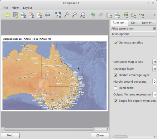
If you are a regular user of QGIS Python plugins, and who isn’t, then you would have used the awesome Atlas plugin developed by Vincent Picavet. This great tool can be used to generate mapbooks, or an atlas as some people like to say, using a coverage layer and a print composer. What makes this even more awesome is that it is now built into the print composer.

Atlas composer intergration

The builtin atlas function also gives you the ability to use an expression to do runtime text replacement, including access to all the fields on the coverage layer.  The coverage layer doesn’t even have to be a region layer, it can be a simple point layer, or even a line layer.   You can see the result of me running the atlas generation from the above example here

Big thanks to Oslandia for integrating this great feature, and the companies sponsoring the work.

New Python console

This new addition comes from the great work that Salvatore Larosa has been doing to add a better Python console to QGIS.

The new Python console includes attribute auto complete, syntax highlighting, better copy and paste, uploading to codepad, the ability to run code from a file, etc.  You don’t realise how much difference there is until you go back to using the old one in version 1.8.

New Python console

Tabbed and groups in builtin forms

One of the things I really loved about QGIS, coming from MapInfo, was the builtin forms.  Just having the ability to enter data using controls like combo boxes, calendar widgets, etc makes you one step closer to having better data.   This feature is the exact reason I setup a 67 year old for kerb data collection.

As good as they are the builtin forms have an issue of ending up with as a big scrolling list with lots of fields; also the lack of  the ability to group or put fields on tabs in the UI meant you had to create a custom form.  Well not any more.

There is now a combo box on the Fields tab that allows you to build a generated form but also add tabs and group boxes.  You can even have the same field shown more then once on the form, handy for something like an ID field that you would like to show on each tab.

With this new ability the builtin forms can get me 95% of the way for data entry jobs, the other 5% I just make a custom form – but that is very rare.

Sextante

Sextante is a great and powerful analytical framework that has been added to the core of QGIS thanks to Victor Olaya.  This is not a feature that I use a lot but this is only due to most of my work being in development and not analysis, however that doesn’t mean that it’s not a really cool feature.

One of the greatest things about the Sextante toolbox is that it allows you to integrate other great open source tools like GRASS, SAGA, R, OTB, etc, right into your QGIS workflow and view the results in the canvas. It even includes a modeller so that you can build a connected diagram of all the bits of your process, even if it crosses between programs.

The toolbox

For me what is even better is that you can use Sextante in your plugins or custom Python code.  Sextante has a Python interface – well the whole thing is written in Python – that you can use to run a Sextante supported algorithm.

import sextante
outputs_0=sextante.runalg("grass:v.crossbones", /file, 0, ,, 1, 2, 3, 4, 1=3.0,2=8.0,5=6.0,8=6.0,11=6.0,14=6.0, None)
outputs_1=sextante.runalg("grass:v.delaunay", outputs_0['output'], True, True, None)
outputs_2=sextante.runalg("grass:v.dissolve", outputs_0['output'], , None)

Victor has created a blog to cover some Sextante recipes at QGIS-SEXTANTE cookbook/. There are also some really cool example of Sextante in use at:

• http://www.qgis.org/en/community/qgis-case-studies/pinhel-portugal.html
• http://www.qgis.org/en/community/qgis-case-studies/lisbon-portugal.html

Massive amount of composer additions

This last feature, or rather feature set,  comes from the sponsorship and support of the World Bank, Australia-Indonesia Facility for Disaster Reduction, Geoscience Australia and the GFDRR.  Most of this work was done to aid in the development of a new QGIS plugin called inaSAFE, which has also received some great praise

“(InaSAFE) is very beneficial for all of us. It’s a good example of our partnership.”
Dr Susilo Bambang Yudhoyono – President of Indonesia

Some of the improvements include:

• A new loadFromTemplate method, in the API, that can do text replacement in the QGIS composer template.
• Better support for EPSG:4326 scale bars
• Multipage in one composer
• Automatic overview frame in map frame
• HTML frame
• Zebra style grid frame border
• More control of grid labels. Inside, outside, disabled
• etc, etc

These are great additions to the QGIS composer and I have already used the overview frame feature along with the new atlas integration  to make some quick nice looking map books. \

A huge thanks to the World Bank, Australia-Indonesia Facility for Disaster Reduction, Geoscience Australia and the GFDRR, and all the developers included.

You can see some of the output that InaSAFE generates using some of these new features at http://quake.linfiniti.com/

P.S The World Bank also sponsored the new raster Save As.. ability just like we have for vector layers.

Last Thursday and Friday was our first local Australian FOSS4G event which was hosted at the CSRIO building in Brisbane.  Very big thanks to CSRIO for hosting the event.  The venue was setup perfectly for  hosting an event like this, including dual projectors for presenting, video calls over to Perth, etc.

The first day was done using a un-conference style of event. This is the first time I’ve been to a un-conference and I liked the format a lot.   Once everyone was there on the first morning we collected ideas from people and everyone voted on which ones they would like to see.  After we had picked enough topics Shaun and I made a program for the day and we started.

Topics included:

• State of GeoServer
• QMap
• CouchDB
• Moblie mapping
• Full open source stacks
• Open Source GIS in Education

Me presenting QMap

The second day was a code sprint.  I worked on converting a MapBasic scripts from one of the guys to QGIS, and Jody enlisted the others to help check the headers of the GeoServer project so that it can finally pass OSGeo incubation.

Overall I think it was a very successful event.  I would like to make these a yearly event if we can, provided that we have people to talk, or projects to work on.

More information about up coming OSGeo events in Australia and New Zealand can be found at http://www.meetup.com/osgeo-aust-nz/

The city of Vienna provides both subdistrict geometries and population statistics. Mapping the city’s population density should be straightforward, right? Let’s see …

We should be able to join on ZBEZ and SUB_DISTRICT_CODE, check! But what about the actual population counts? Unfortunately, there is no file which simply lists population per subdistrict. The file I found contains four lines for each subdistrict: females 2011, males 2011, females 2012 and males 2012. That’s not the perfect format for mapping general population density.

A quick way to prepare our input data is applying pivot tables, eg. in Open Office: The goal is to have one row per subdistrict and columns for population in 2011 and 2012:

Export as CSV, add CSVT and load into QGIS. Finally, we can join geometries and CSV table:

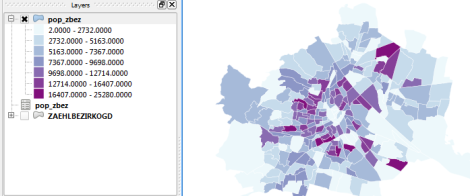
A quick look at the joined data confirms that each subdistrict now has a population value. But visualizing absolute values results in misleading maps. Big subdistricts with only average density will overrule smaller but much denser subdistricts:

That’s why we need to calculate population density. This is easy to do using Field Calculator. The subdistrict file already contains area values but even if they were missing, we could calculate it using the $area operator: "pop2012" / ($area / 10000). The resulting population density in population per ha finally shows which subdistricts are the most densely populated:

One could argue that this is still no accurate representation of population density: Big parts of some subdistricts are actually covered by water – especially along the Danube – and therefore uninhabited. There are also big parks which could be excluded from the subdistrict area. But that’s going to be the topic of another post.

If you want to use my results so far, you can download the GeoJSON file from Github.