Related Plugins and Tags

QGIS Planet

QGIS Layer Tree API (Part 3)

In the two previous blog posts we have learned how to query a layer tree and how to modify it. All these new APIs are available since QGIS 2.4 release. Today we will look into how to make layer trees available in GUI and connect them with a map canvas.

Model/View Overview

As we have seen earlier, a layer tree is a usual hierarchical data structure composed from nodes of two types - layers and groups. They do not provide any GUI functionality as they live in the QGIS core library. In order to visualize a layer tree, we will use Model/View approach from Qt framework. Readers not familiar with those concepts are recommended to read the Qt Model/View overview first.
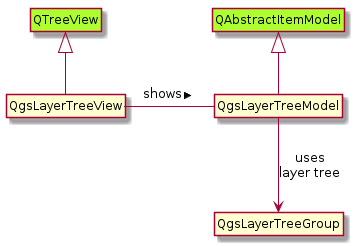
Layer tree model/view

There is QgsLayerTreeModel class (derived from QAbstractItemModel) which as you may have guessed provides a model to access a layer tree. Instance of this class may be used in any QTreeView class, however it is recommended to use it together with QgsLayerTreeView because of the extra convenience functionality offerred by the custom view class.

Here is an example how to create another view of current project’s layer tree (try that in QGIS Python console):

from qgis.gui import *

root = QgsProject.instance().layerTreeRoot()
model = QgsLayerTreeModel(root)
view = QgsLayerTreeView()
view.setModel(model)
view.show()

Any changes that happen to the layer tree structure are automatically monitored by the model/view classes. After running the example above, try changing a layer’s name or add/remove/reorder some layers - all those actions will be immediately visible in all views.

As you can see, the layer tree view is just one way how to visualize the underlying layer tree - in the future it may be possible to have different ways to show the layer tree, for example using Qt’s QML framework (with all sorts of animated transitions known from mobile apps).

Plugin developers can access the layer tree view in the main window of QGIS through the following interface call:

view = iface.layerTreeView()

More About the Model

The model is meant to be flexible and it is possible to use it in various contexts. For example, by default the model also provides legend for the layers in the tree. This however may not be wanted in some cases. Similarly, sometimes the layer tree should be read-only while in other context it is desired that the user can reorder layers or change their names. These preferences can be passed to the model with flags:

model = QgsLayerTreeModel(root)
model.setFlag(QgsLayerTreeModel.AllowNodeReorder)
model.setFlag(QgsLayerTreeModel.AllowNodeChangeVisibility)

The setFlag() method has optional second parameter “enabled” (True by default). Flags can be also set all at once with setFlags() method which expects a combination of flags joined by binary OR operator. There are also flags() and testFlag() methods to query the current flags.

The QgsLayerTreeModel class also provides routines for conversion between QgsLayerTreeNode instances and corresponding QModelIndex objects used by Qt Model/View framework - index2node() and node2index() may come handy especially when working with views.

There is also some functionality related to legend display - it has been greatly extended in QGIS 2.6 release and we will try to cover that in a future blog post.

More About the View

As mentioned earlier, it is possible to use any QTreeView instance in combination with QgsLayerTreeModel to show the layer tree, but it is highly recommended to use QgsLayerTreeView class (a subclass of QTreeView) because of the additional functionality it provides (and more may be added in the future):

  • Easier handling of selection. Normally one needs to work with selection through view’s selection model. The QgsLayerTreeView class adds higher level methods that operate with QgsLayerTreeNode objects like currentNode() or with QgsMapLayer objects like currentLayer().

    def onChange(layer):
      QMessageBox.information(None, "Change", "Current Layer: "+str(layer))
    
    # connect to the signal
    view.currentLayerChanged.connect(onChange)
    # change selection to the top-most layer (onChange will be also called)
    view.setCurrentLayer( iface.mapCanvas().layers()[0] )
    
  • Display of context menu. It is possible to assign a menu provider to the view (subclass of QgsLayerTreeViewMenuProvider) - its createContextMenu() implementation will return a QMenu object with custom actions whenever user right-clicks in the view. Additionally, there is a factory class QgsLayerTreeViewDefaultActions that can create commonly use actions for use in the menu, such as “Add Group”, “Remove” or “Zoom to Layer”. The following example shows how to create a provider with one action that shows the current layer’s extent:

    class MyMenuProvider(QgsLayerTreeViewMenuProvider):
      def __init__(self, view):
        QgsLayerTreeViewMenuProvider.__init__(self)
        self.view = view
    
      def createContextMenu(self):
        if not self.view.currentLayer():
          return None
        m = QMenu()
        m.addAction("Show Extent", self.showExtent)
        return m
    
      def showExtent(self):
        r = self.view.currentLayer().extent()
        QMessageBox.information(None, "Extent", r.toString())
    
    provider = MyMenuProvider(view)
    view.setMenuProvider(provider)
    

Interaction with Canvas

The layer tree classes and map canvas class are separate components that are not dependent on each other. This is a good thing and a great step forward, because until QGIS 2.2 there was big internal monolithic QgsLegend view class that handled everything and it was directly connected to map canvas and various other components, making it impossible to reuse it elsewhere. With the new layer tree API this has been solved, now it is possible use map canvas without an associated layer tree view or vice versa - to use a layer tree view without map canvas. It is even possible to get creative and use one layer tree with several map canvas instances at once.

Layer tree and map canvas can be connected via QgsLayerTreeMapCanvasBridge class. It listens to signals from the given layer tree hierarchy and updates canvas accordingly. Let’s see how we could create a new map canvas that would show the same layers as the main canvas does:

canvas = QgsMapCanvas()
root = QgsProject.instance().layerTreeRoot()
bridge = QgsLayerTreeMapCanvasBridge(root, canvas)
canvas.zoomToFullExtent()
canvas.show()

That’s it! We have tied the new canvas with project’s layer tree. So any actions you do in the layer tree view (for example, add or remove layers, enable or disable layers) are automatically passed to the new canvas. And of course this does not work just with project’s layer tree - you could use any custom layer tree in your layer tree model/view or canvas.

The bridge class has advanced functionality worth mentioning. By default the ordering of layers in canvas is according to the order in the layer tree (with first layer in the tree being at the top), though there are API methods to override the default order.

For convenience, the bridge by default also configures some settings of the canvas (this can be disabled if necessary):

  • enable on-the-fly reprojections if layers have different coordinate reference system (CRS)
  • setup destination CRS and map units when first layers are added
  • zoom to full extent when first layers are added

Summary

I hope you have enjoyed the three blog posts introducing QGIS layer tree API. They should cover everything you need to know in order to start using the new functionality. In a future post we will have a look at the new legend API that nicely complements the layer tree API - stay tuned!

You may also like...

Mergin Maps, a field data collection app based on QGIS. Mergin Maps makes field work easy with its simple interface and cloud-based sync. Available on Android, iOS and Windows. Screenshots of the Mergin Maps mobile app for Field Data Collection
Get it on Google Play Get it on Apple store

New addition

Stace and I would like to welcome Matilda Anne Woodrow, born 5/1/15 at 10:36am.

Matilda

She is a nice way to start 2015.

After the pretty crappy year that was 2014 it was finally nice to see Matilda in the flesh. The relief of seeing her alive and well is hard to put in words after losing Ellie in 2013.

People always ask about the lack of sleep, but it feels like we have more energy now then we did before. The emotional and physical toll that the pregancy took on our family had pretty much run us into the ground and it felt like it was never ending.

The toll of the pregancy had lead me to massive lack of motivation towards QGIS and pretty much everything else in life, which isn't healthy when you have a family to look after. Pro Tip: Get help if you find yourself in this spot, it be hard to recover if you go over the edge.

Anyway. Here is to a new year. A better year.

Function editor for QGIS expressions

A new feature for QGIS 2.8 is a function editor for expressions. Being able to define your own custom functions has be possible for a while now, over a year, I even have a plugin (Expressions+) that adds some extra ones, however it wasn’t easy for new users and required you to create files that lived on python path while also editing the startup.py file for QGIS so that functions got registed at start up. Way too much effort for my liking.

This feature is now exposed via the expression builder on the Function Editor tab. The function editor will create new Python files in qgis2\python\expressions and will auto load all functions defined when starting QGIS. I remember Sean Gillies saying that Python support in a field calculator should be a gateway to full Python programming, can’t get any more Python then full Python modules.

The best way to show this feature is a quick video so here it is

The play button in the editor will run the current editor file in the QGIS session and register any functions it finds, it will also save the file in the expressions folder.

You can make a new file by pressing the new file button which will add the basic function template, changing the name in the combobox and hitting save will save the file.

The function editor allows you have to define reuseable functions for your QGIS. If you want to share a function you simply share the .py file from the expressions folder and give it to another user. In future versions of QGIS we might have a way to download other users functions.

Auto expanding values

You can also use the args="auto" keyword in place of the number of args which will let QGIS work it out and expand the arguments for you.

Here is an example

@qgsfunction(args="auto", group='Custom')
def myfunc(value1, value2 feature, parent):
    pass

and can be used like this:

myfunc('test1', 'test2')

QGIS will workout how many arguments your function takes based on what you have defined. Note: The last arguments should always be feature, parent, these are not included in the count.

Raising errors

If you need to report a error from a function simply use the raise method like normal in QGIS and raise an exception.

@qgsfunction(args="auto", group='Custom')
def myfunc(value1, value2 feature, parent):
    raise Expection("Hahah Nope!")

The function wrapper will catch the exception and raise it though the expression engine.

A couple of things to note

  • New functions are only saved in the expressions folder and not in the project file. If you have a project that uses one of your custom functions you will need to also share the .py file in the expressions folder.
  • The editor doesn’t unregister any functions. If you define a function called test, hit play, change the name to test_2, hit play, both functions will exist until you reload QGIS.

Filed under: Open Source

Function editor for QGIS expressions

A new feature for QGIS 2.8 is a function editor for expressions. Being able to define your own custom functions has be possible for a while now, over a year, I even have a plugin (Expressions+) that adds some extra ones, however it wasn't easy for new users and required you to create files that lived on python path while also editing the startup.py file for QGIS so that functions got registed at start up. Way too much effort for my liking.

This feature is now exposed via the expression builder on the Function Editor tab. The function editor will create new Python files in qgis2\python\expressions and will auto load all functions defined when starting QGIS. I remember Sean Gillies saying that Python support in a field calculator should be a gateway to full Python programming, can't get any more Python then full Python modules.

The best way to show this feature is a quick video so here it is

The play button in the editor will run the current editor file in the QGIS session and register any functions it finds, it will also save the file in the expressions folder.

You can make a new file by pressing the new file button which will add the basic function template, changing the name in the combobox and hitting save will save the file.

The function editor allows you have to define reuseable functions for your QGIS. If you want to share a function you simply share the .py file from the expressions folder and give it to another user. In future versions of QGIS we might have a way to download other users functions.

Auto expanding values

You can also use the args="auto" keyword in place of the number of args which will let QGIS work it out and expand the arguments for you.

Here is an example

@qgsfunction(args="auto", group='Custom')
def myfunc(value1, value2 feature, parent):
    pass

and can be used like this:

myfunc('test1', 'test2')

QGIS will workout how many arguments your function takes based on what you have defined. Note: The last arguments should always be feature, parent, these are not included in the count.

Raising errors

If you need to report a error from a function simply use the raise method like normal in QGIS and raise an exception.

@qgsfunction(args="auto", group='Custom')
def myfunc(value1, value2 feature, parent):
    raise Expection("Hahah Nope!")

The function wrapper will catch the exception and raise it though the expression engine.

A couple of things to note

  • New functions are only saved in the expressions folder and not in the project file. If you have a project that uses one of your custom functions you will need to also share the .py file in the expressions folder.
  • The editor doesn't unregister any functions. If you define a function called test, hit play, change the name to test_2, hit play, both functions will exist until you reload QGIS.

Labels leading lines with QGIS and Postgis

EN | PT

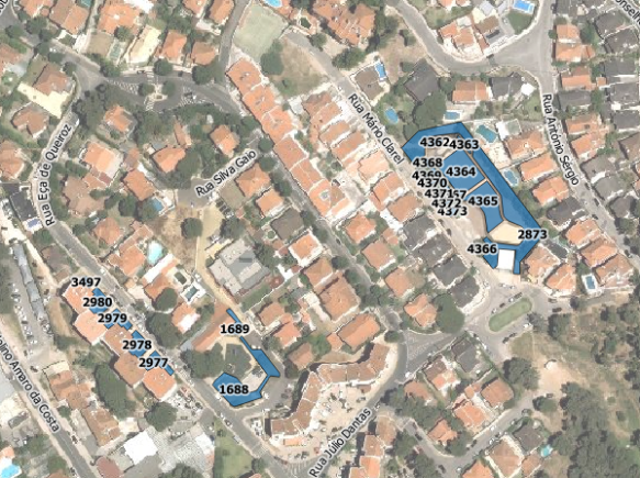
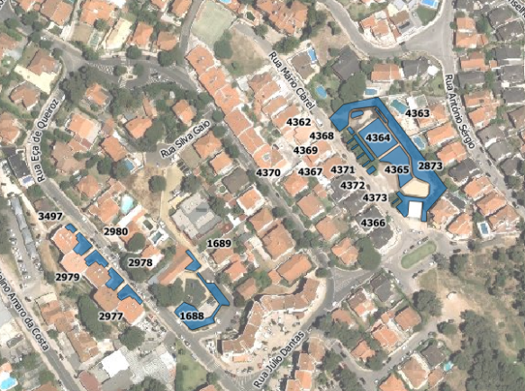
Recently I had the need to add labels to features with very close geometries, resulting in their collision.

Capturar_3

Using data-defined override for label’s position (I have used layer to labeled layer plugin to set this really fast) and the QGIS tool to move labels, it was quite easy to relocate them to better places. However, in same cases, it was difficult to understand to which geometry they belonged.

Capturar_2

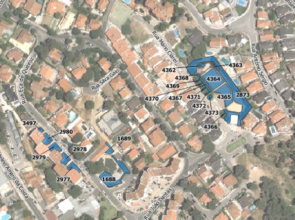
I needed some kind of leading lines to connect, whenever necessary, label and feature. I knew another great plugin called “Easy Custom Labeling“, by Regis Haubourg, that did what I needed, but it would create a memory duplicate of the original layer, wish meant that any edition on the original layer wouldn’t be updated in the labels.

Since the data were stored in a PostgreSQL/Postgis database, I have decided to create a query that would return a layer with leading lines. I used the following query in DB manager:

SELECT
  gid,
  label,
  ST_Makeline(St_setSRID(ST_PointOnSurface(geom),27493), St_setSRID(St_Point(x_label::numeric, y_label::numeric),27493))
FROM
  epvu.sgev
WHERE
  x_label IS NOT NULL AND
  y_label IS NOT NULL AND
  NOT ST_Within(ST_Makeline(St_setSRID(ST_PointOnSurface(geom),27493), St_setSRID(St_Point(x_label::numeric, y_label::numeric),27493)),geom))

This query creates a line by using the feature centroid as starting point and the label coordinate as end point. The last condition on the WHERE statement assures that the lines are only created for labels outside the feature.

Capturar_1

With the resulting layer loaded in my project, all I need is to move my labels and save the edition (and press refresh) to show a nice leading line.

guidelines

A line gradient style hack

Today’s post was motivated by a question over on gis.stackexchange, basically: How to draw a line with a gradient?

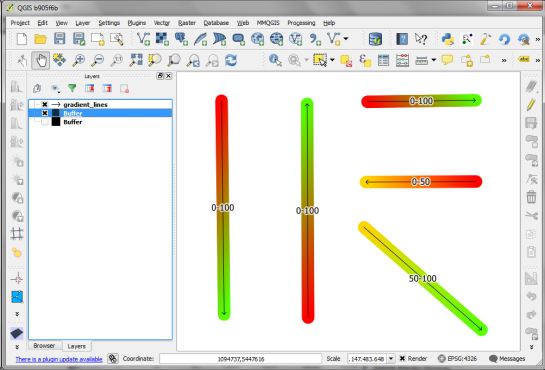
The issue we have to deal with is there is no gradient line style yet … But there are polygon gradient fills. So we can buffer the line and style the buffers. It’s a bit of an exercise in data-defined styling though:

Screenshot 2015-01-11 22.49.41

Before creating the buffer layer, we need to add the coordinates of the line start and end node to the line attributes. This is easy to do using the Field Calculator functions xat and yat, for example xat(0) for the x coordinate of the start node and yat(-1) for the y coordinate of the end node.

Screenshot 2015-01-11 22.41.37

Then we can buffer the lines and start styling the buffers. As mentioned, we’ll use the Gradient fill Symbol layer type.

Screenshot 2015-01-11 22.49.54

The interesting part happens in the Data-defined properties. The start and end colors are computed from the measurement values from_m and to_m. Next, it’s important to use the feature coordinate mode because this will ensure that the coordinate system for the color gradient is based on the feature extent (with [0,0] in the upper left corner of the feature bbox).

Once that’s set up, we can compute the gradient start and end positions based on the line start and end node locations which we added to the attribute table in the beginning. If you’re wondering why Reference point 1 y is based on to_y (y coordinate of the line end point) rather than from_y, it’s due to the difference in coordinate origins in the geometry and the color gradient coordinate space: [0,0] is the lower left corner for the geometries but the upper left corner for the color gradient.

Screenshot 2015-01-11 22.42.35

As the title suggests, this is a really hackish solution for gradient line symbols. It will only provide reasonable results for straight – or close to straight – lines. But I’m very confident that we’ll have a real gradient line style in QGIS sooner or later.


QGIS – live layer effects Kickstarter update

Here’s another quick video demonstration of the latest developments in layer effects – effects on polygon and polyline layers, and outer glow effects:

Time is running out to fund this campaign and make this work happen… Please donate via Kickstarter!

I’ve also been asked what will happen if funding exceeds the Kickstarter goal? Well, if this happens, the extra funds will be used to add additional layer effects to QGIS. Next up will be inner glow, inner shadow and color modification effects.

New addition

Stace and I would like to welcome Matilda Anne Woodrow, born 5/1/15 at 10:36am.

tilly

She is a nice way to start 2015.

After the pretty crappy year that was 2014 it was finally nice to see Matilda in the flesh. The relief of seeing her alive and well is hard to put in words after losing Ellie in 2013.

People always ask about the lack of sleep, but it feels like we have more energy now then we did before. The emotional and physical toll that the pregancy took on our family had pretty much run us into the ground and it felt like it was never ending.

The toll of the pregancy had lead me to massive lack of motivation towards QGIS and pretty much everything else in life, which isn’t healthy when you have a family to look after. Pro Tip: Get help if you find yourself in this spot, it be hard to recover if you go over the edge.

Anyway. Here is to a new year. A better year.


Filed under: Open Source

Use of the Flemish geographical data portal Geopunt in QGIS

Geopunt website Geopunt is the central portal for geographical data of the Flemish government. Beside an online viewer, a catalogue is available from where data can be downloaded. A lot of these data are free to download (e.g. orthophotos), other data is available depending on your user profile (e.g. soil map) Download through the Geopunt4Qgis … Continue reading Use of the Flemish geographical data portal Geopunt in QGIS

How to: watercolor pastel style in QGIS

Today’s post is a follow-up to a recent map experiment which I published in the QGIS Flickr group. It’s basically an inverted Stamen Toner style with an image in the map composition background instead of a solid color (similar to the approach described for vintage maps):

That’s nice but with this approach we only get to enjoy the complete design in the print composer but not in the main window. So what other options do we have? – SVG fills to the rescue!

But first we need a suitable SVG with this nice pastel style. I used Gimp to create a seamless version of the pastel image and then embedded the image in an SVG using Inkscape:

LT_RemixedChalkPastel_snakk_seamless

In QGIS, this SVG can now be used in any SVG fill. It’s important to set the Texture width setting to a quite high value when working with SVGs containing big textures, otherwise the images will be rendered very small and the repeating patterns will be very obvious.

Screenshot 2015-01-04 17.49.11

Once the background is in place, we can add the line work and labels. The roads are white with black outlines for bridges which – together with the Lighten blending mode – produce the desired effect:

Screenshot 2015-01-04 17.37.33


Happy new year!

Thank you for a great 2014! It’s been a pleasure to see the open source GIS community grow and experience what we can create together. It’s great to see the interest for open source GIS all over the world:

In total, this blog has been visitied from 216 countries. Most visitors came from The United States. Germany & France were not far behind.

In total, this blog has been visitied from 216 countries. Most visitors came from The United States. Germany & France were not far behind.

Since my first post in 2010, the development of this blog has exceeded all expectations I might have had by far. For 2014, the WordPress blog view counter shows a staggering 330,000 views or over 900 views per day.

In case you were wondering, the most popular posts of 2014 were:

  1. 3D Viz with QGIS & three.js
  2. A guide to GoogleMaps-like maps with OSM in QGIS
  3. A QGIS 2.2 preview
  4. Getting started writing QGIS 2.x plugins
  5. and Toner-lite styles for QGIS

Thank you, your feedback has been a continuous source of motivation. All the best for 2015!


Top10 QGIS Planet posts 2014

It’s the end of December and time to recap 2014. Therefore, I decided to have a look at what this year has brought us. There were plenty of great posts for both casual and power users as well as developers. Here is my pick of the top 10 posts from the QGIS Planet blog aggregator.

  1. Tons of colour improvements! (Nyall Dawson)
  2. The QGIS Field calculator is dead. Long live the Field calculator bar (Nathan Woodrow)
  3. Why QGIS Class Names Start with Qgs (Gary Sherman)
  4. Atlas Previews (Nyall Dawson)
  5. QGIS atlas on non geometry tables (Nathan Woodrow)
  6. Gradient Fills (Nyall Dawson)
  7. What are all these QGIS file types? Why do I need them (Nathan Woodrow)
  8. Getting Started Writing QGIS Python Plugins (Peter Wells)
  9. QGIS Layer Tree API (Martin Dobias)
  10. Shapeburst fill styles (Nyall Dawson)

More great features and posts are sure to come next year. For example, Nyall is currently running a campaign on Kickstarter to add Live Layer Effects such as drop shadow effects to QGIS. Please support it if you can.


Kickstarter Alert – Live Layer Effects for QGIS

QGIS is well regarded for its fantastic cartographic abilities – it’s got a huge range of symbology styles and options which can be used to style your maps. But there’s more we can do to push this even further.

One long requested cartographic feature has been for live drop shadows on layers. Why stop there? Why not inner and outer glow effects and live blur effects? Just imagine the cartographic possibilities if this functionality was available from within a GIS, and didn’t require exporting maps to external editors…

I’ve launched a Kickstarter project to fund implementing live layer effects like this within QGIS. Please consider donating or spreading the word if you’d find this feature useful!

Exploring open government population data collected by ODVIS-AT

At FOSS4G2013, I had the pleasure to attend a presentation about the ODVIS.AT project by Marius Schebella from the FH Salzburg. The goal of the project – which ended in Summer 2014 – was “to display open data (demographic, open government data) in a quick and easy way to end users” by combining it with OpenStreetMap. Even though their visualization does not work for me (“unable to get datasets” error), not all is lost because they provide an SQL dump of their PostGIS database.

Checking the data, it quickly becomes apparent that each data publisher decided to publish a slightly different dataset: some published their population counts as timelines over multiple years, others classified population by migration background, age, or gender. Also, according to the metadata table, no data from Salzburg and Burgenland were included. Most datasets’ reference date is between 2011 and 2013 but the data of the westernmost state Vorarlberg seems to be from 2001.

Based on this database, I created a dataset combining the municipalities with the Viennese districts and joined the population data from the individual state tables. The following map shows the population density based on this dataset: it is easy to recognize the densely populated regions around Vienna, Linz, Graz, and in the big Alpine valleys.

odvis_popdens

Overall, it is incredibly time-consuming to create this seemingly simple dataset. It would be very helpful if the publishers would agree on a common scheme for releasing at least the most basic information.

Considering that OpenStreetMap already contains population data, it barely seems worth all the trouble to merge these OGD datasets. Granted, the time lines of population development would be interesting but they are not available for each state.

P.S. If anyone is interested in the edited database, I would be happy to share the SQL dump.


Shortcuts to hide/show panels in QGIS

Just a quick one to show how to assign shortcuts to hide and show for panels in QGIS. Add this to your .qgis2\python\startup.py

from functools import partial
from qgis.utils import iface

from PyQt4.QtCore import *
from PyQt4.QtGui import *

mappings = {"Layers": Qt.ALT + Qt.Key_1,
            "Browser": Qt.ALT + Qt.Key_2,
            "PythonConsole": Qt.ALT + Qt.Key_3}
shortcuts = []

def activated(dock):
    dock = iface.mainWindow().findChild(QDockWidget, dock)
    visible = dock.isVisible()
    dock.setVisible(not visible)

def bind():
    for dock, keys in mappings.iteritems():
        short = QShortcut(QKeySequence(keys), iface.mainWindow())
        short.setContext(Qt.ApplicationShortcut)
        short.activated.connect(partial(activated, dock))
        shortcuts.append(short)

bind()

and now you can hide and show using ALT + number


Filed under: Open Source

Shortcuts to hide/show panels in QGIS

Just a quick one to show how to assign shortcuts to hide and show for panels in QGIS. Add this to your .qgis2\python\startup.py

from functools import partial
from qgis.utils import iface

from PyQt4.QtCore import *
from PyQt4.QtGui import *

mappings = {"Layers": Qt.ALT + Qt.Key_1,
            "Browser": Qt.ALT + Qt.Key_2,
            "PythonConsole": Qt.ALT + Qt.Key_3}
shortcuts = []

def activated(dock):
    dock = iface.mainWindow().findChild(QDockWidget, dock)
    visible = dock.isVisible()
    dock.setVisible(not visible)

def bind():
    for dock, keys in mappings.iteritems():
        short = QShortcut(QKeySequence(keys), iface.mainWindow())
        short.setContext(Qt.ApplicationShortcut)
        short.activated.connect(partial(activated, dock))
        shortcuts.append(short)

bind()

and now you can hide and show using ALT + number

2nd edition of Learning QGIS

It’s my pleasure to announce that the updated and extended 2nd edition of Learning QGIS is available now.

I also want to take this opportunity to thank everyone who made the 1st edition such a great success!

This second edition has been updated to QGIS 2.6 and it features a completely new 6th chapter on Expanding QGIS with Python. It introduces the QGIS Python Console, shows how to create custom Processing tools, and provides a starting point for developing plugins.

Overall, the book has grown by 40 pages and the price of the print version has dropped by 3€ :-)

Happy QGISing!

2031OSos_mockupcover_normal_0


GRASS GIS 7: Vector data reprojection with automated vertex densification

GRASS GIS 7 just got better: When reprojecting vector data, now automated vertex densification is applied. This reduces the reprojection error for long lines (or polygon boundaries). The needed improvement has been kindly added in v.proj by Markus Metz.

1. Example

As an (extreme?) example, we generate a box in LatLong/WGS84 (EPSG: 4326) which is of 10 degree side length (see below for screenshot and at bottom for SHAPE file download of this “box” map):

[neteler@oboe ~]$ grass70 ~/grassdata/latlong/grass7/
# for the ease of generating the box, set computational region:
g.region n=60 s=40 w=0 e=30 res=10 -p
projection: 3 (Latitude-Longitude)
zone:       0
datum:      wgs84
ellipsoid:  wgs84
north:      60N
south:      40N
west:       0
east:       30E
nsres:      10
ewres:      10
rows:       2
cols:       3
cells:      6
# generate the box according to current computational region:
v.in.region box_latlong_10deg
exit

Next we start GRASS GIS in a metric projection, here the EU LAEA:

# EPSG 3035, metric EU LAEA:
grass70 ~/grassdata/europe_laea/user1/
GRASS 7.0.0svn (europe_laea): >

Now we first reproject the map the “traditional way” (no vertex densification as in most GIS, here enforced by smax=0):

v.proj box_latlong_10deg out=box_latlong_10deg_no_densification
location=latlong mapset=grass7 smax=0

Then we do a second reprojection with new automated vertex densification (here we use the default values for smax which is a 10km vertex distance in the reprojected map by default):

v.proj box_latlong_10deg out=box_latlong_10deg_yes_densification
location=latlong mapset=grass7

Eventually we can compare both reprojected maps:

g.region vect=box_latlong_10deg_no_densification

# compare:
d.mon wx0
d.vect box_latlong_10deg_no_densification color=red
d.vect box_latlong_10deg_yes_densification color=green fill_color=none
Comparison of the reprojection of a 10 degree large LatLong box to the metric EU LAEA (EPSG 3035): before in red and new in green. The grid is based on WGS84 at 5 degree spacing.

Comparison of the reprojection of a 10 degree large LatLong box to the metric EU LAEA (EPSG 3035): before in red and new in green. The grid is based on WGS84 at 5 degree spacing.

The result shows how nicely the projection is now performed in GRASS GIS 7: the red line output is old, the green color line is the new output (its area filling is not shown).

Consider to benchmark this with other GIS… the reprojected map should not become a simple trapezoid.

2. Sample dataset download

Download of box_latlong_10deg.shp for own tests (1kB).

The post GRASS GIS 7: Vector data reprojection with automated vertex densification appeared first on GFOSS Blog | GRASS GIS Courses.

  • <<
  • Page 71 of 142 ( 2821 posts )
  • >>

Back to Top

Sustaining Members