Related Plugins and Tags

QGIS Planet

How to do X in QGIS

A great new initiative has been started on QGIS wiki: “How to do X in QGIS” aims at providing step-by-step tutorials for various tasks based on the latest versions of QGIS. This new knowledge base is meant to complement the existing documentation and to replace some of the outdated tutorials available all over the web.

Feel free to contribute tutorials or tutorial ideas, it’s a wiki!


Picking a Feature’s Attribute Value From a WMS Layer With OpenLayers

There are many nice examples out there of how to use a getFeatureInfo request in OpenLayers to display a feature’s attribute table. In some applications it can be useful though not to display the full attribute table but to only select one attribute value from it and output it somewhere, e.g. in a text field.

This post describes how to pick the road id from a road wms layer and write the id value into a text input field.

OpenLayers offers a convenient class to achieve this: OpenLayers.Control.WMSGetFeatureInfo.

Let’s create an object of this class, register and activate it:

roadidPicker = new OpenLayers.Control.WMSGetFeatureInfo({
                url: 'http://localhost:8080/geoserver/wms',
                title: 'identify features on click',
                layers: [wms],
                queryVisible: true
            });
roadidPicker.infoFormat = 'application/vnd.ogc.gml';
roadidPicker.events.register("getfeatureinfo", this, pickRoadid);
map.addControl(roadidPicker);
roadidPicker.activate();

Now, every time the user clicks onto the map, a getFeatureInfo request is issued and the function pickRoadid() is called. In pickRoadid(), we’ll define which value we want to pick from the feature. The ‘id’ of the feature will be written into a text input field called ‘roadId’:

function pickRoadid(e) {
  if (e.features && e.features.length) {
     var val = e.features[0].attributes.id;
     document.getElementById('roadId').value = val;
  }
}

You might have noticed the ‘[0]‘. That’s because the click event comes with a list of features within the reach of the mouse click. For my application, I can only use one value and the first feature in this list is as good as any.


Opening MS SQL Server 2008 Spatial tables in QGIS

EDIT:  If you are having trouble opening MS SQL 2008 in QGIS I will have a blog post coming explaining how to correct it. Or you can read the comments between TheGeoist and I below which will have the answer.

Just a quick tip.

Thanks to GDAL/OGR 1.8 QGIS can now open MS SQL Server 2008 spatial tables via the OGR MSSQLSpatial driver.

First you must be running a version of QGIS that is using GDAL/OGR 1.8.  Opening the QGIS about page will tell you if it is supported.

Need version 1.8 or higher

As I am writing this on my Ubuntu install I only have version 1.6.3 but the latest dev version of QGIS (upcoming 1.7 release) for Windows in the OSGeo4W installer is complied with version 1.8.

Now open the python console in QGIS and type the following:

uri = "MSSQL:server={serverName};database={databaseName};tables={tableName};trusted_connection=yes"
qgis.utils.iface.addVectorLayer(uri,'{yourLayerNameHere}','ogr')

Replacing {serverName} with your server name, if installed on your local machine you can use localhost; {databaseName} with the name of the database with the tables;{tableName} with the table to open; {yourLayerNameHere} with the name you would like the layer to have in the map legend.

After that you should see your MS SQL Spatial table displayed in QGIS, with editing support.

At the moment there is no nice interface in QGIS to open MS SQL tables like there is for PostGIS, although that might be a good plugin project for someone to work on.


Filed under: Open Source, qgis Tagged: gis, mapping, MS SQL Server 2008, MS SQL Spatial, Open Source, OSS, python, qgis, Quantum GIS

How to Label Only Selected Features in QGIS

The aim of this post is to describe a method for labeling of a subset of features within a layer using new labeling functionality.

The problem

Often, we want to label only a few features in a layer. Of course we can export those features to a new layer and label them that way, but that requires creation of additional files and layers within your project. Things will start to get messy fast.

Another approach is to delete unwanted label texts from the attribute table. This either means that you have to duplicate a “name” attribute and then start deleting from the newly created attribute table column or that you actually delete values in the original column. Both approaches are problematic. Either you produce redundancy that gets difficult to maintain (two attributes have to be updated if the name of a feature changes) or you loose information from the attribute table.

The suggested solution

Let me present a different approach using new labeling tools. The idea is based on moving unwanted labels out of view. This approach avoids duplication of features and duplication/deletion of label texts. And this is the workflow:

  1. Select the features you want to label
  2. Open attribute table
  3. If you don’t have label attributes ready yet: Add two type “real” columns called e.g. “label_x” and “label_y”
  4. Invert the selection (3rd button in attribute table window)
  5. Open field calculator and fill “label_x” and “label_y” fields of the selected features with 0 values (or any coordinates outside your map extent)
  6. Close field calculator and attribute table
  7. Save your edits
  8. Open the labeling dialog and set “data defined settings” – “x coordinate” and “y coordinate”
  9. Enable “Label this layer” and specify the label field
  10. Done

If you change your mind about a feature and want to label it later on: Simply delete the values in “label_x” and “label_y” fields (so they read NULL).

This works quite well for me but I’m aware that it’s still not optimal. Another “data defined setting” like “show this label (true/false)” would be more intuitive.

Have you found better solutions to this problem? Please, post them!


Getting ECW and MrSID support working in QGIS dev OSGeo4W install

Note:  This post is about getting ecw and mrsid support working in the trunk (qgis-dev) version of QGIS which is installed with the OSGeo4W installer.  Non-dev versions seem to work fine following this method: http://www.qgis.org/wiki/OSGeo4wSetup#Installing_support_for_raster__.2A.ECW_.28ERMapper.29_and_.2A.sid_.28MrSid.29_formats

Getting ECW and MrSID support into QGIS can be a real pain in the butt when you first try; but once you know how it’s easy.

If you try to open a ecw file in QGIS you will get this nice little error message:

What?  I thought QGIS supported ECW files!

Turns out it does, but the team are not able to ship the required libs with the program due to licensing restrictions by ERDAS.   Luckily adding support is not “too” hard.

  1. First head over to http://www.erdas.com/products/ERDASECWJPEG2000SDK/Downloads.aspx
  2. Click Download Now for the ERDAS ECW/JP2 SDK Desktop Read-Only, Version 4.1 libs,
  3. Fill out a bit of registration details and click though all the pages (this is the most painful process I have ever had to go though to get some libs for a program, ERDAS should be ashamed that it is such an effort.)
  4. Once you have download ECWJP2SDKSetup_RO_20100920.exe; install it.
  5. Copy all the files from C:\Program Files\ERDAS\ERDAS ECW JPEG2000 Read SDK\bin\vc90\win32 into the bin folder of your OSGeo4W install (default is C:\OSGeo4W\bin)
    You can open the OSgeo4W shell and run: copy “C:\Program Files\ERDAS\ERDAS ECW JPEG2000 Read SDK\bin\vc90\win32\*.dll” %OSGEO4W_ROOT%\bin to do the same thing.
  6. Launch osgeo4w-setup.exe, the installer that you used to install qgis-dev,  and select  gdal-ecw, gdal17-ecw and gdal-mrsid, gdal17-sid under the libs section. Let it install the needed libs and any dependencies.
  7. Open %OSGEO4W_ROOT%\bin and search for qgis-dev.bat; open it with a text editor and add the following line:
    set GDAL_DRIVER_PATH=”%OSGEO4W_ROOT%”\bin\gdalplugins\1.8
    I always insert it just after  SET OSGEO4W_ROOT=
  8. Launch qgis-dev.bat
  9. Open a ecw

ECW file opened in QGIS

I have tested this on a couple of machines now but as always

with no guarantee that it will work on yours :)  (Although it should)


Filed under: Open Source, qgis Tagged: ecw, gis, mapping, mrsid, Open Source, qgis, Quantum GIS, raster

How to Specify Data Types of CSV Columns for Use in QGIS

If you load .csv files through “Add vector layer”, all columns are interpreted as strings. That’s most likely not what you want, but it’s OGR’s default behaviour:

The OGR CSV driver returns all attribute columns with a type of string if no field type information file (with .csvt extension) is available.

Let’s create a .csvt file then!

The .csvt file has to have the same name as the .csv file it describes. (Same concept used in shapefiles.) It enables definition of the following data types: Integer, Real, String, Date (YYYY-MM-DD), Time (HH:MM:SS+nn) and DateTime (YYYY-MM-DD HH:MM:SS+nn).

A .csvt file contains only one line and the types for each column have to be quoted and comma separated, e.g.

"Integer","Real","String"

You can even specify width and precision of each column, e.g.

"Integer(6)","Real(5.5)","String(22)"

Read more at: www.gdal.org/ogr/drv_csv.html


MapInfo map control into Qt Python form

Tonight for a bit of fun, or shits and jiggles as we say here, I thought I would try and embed a MapInfo map control into a Qt python widget (although I should be studying, but it’s Saturday night) .

Turns out it is pretty easy!

pls send me teh codez? OK here you go.

from PyQt4.QtCore import *
from PyQt4.QtGui import *
from win32com.client import Dispatch
import sys

app = QApplication(sys.argv)
app.setAttribute(Qt.AA_NativeWindows,True)
wnd = QMainWindow()
wnd.resize(400, 400)
widget = QWidget()
wnd.setCentralWidget(widget)
wnd.show()

handle = int(widget.winId())
mapinfo = Dispatch("MapInfo.Application")
mapinfo.do('Set Next Document Parent %s Style 1' % handle)
mapinfo.do('Open Table "D:\GIS\MAPS\Property.TAB"')
mapinfo.do('Map from Property')

app.exec_()

The above code will load MapInfo and open the property layer into the Qt Widget control, with the result below.

MapInfo map in python Qt based form

So this means you don’t “always” have to write your MapInfo based apps in C# or C++; of course I already knew this as anything that can use OLE and provide a native window handle to MapInfo will work, I just never tried it.


Filed under: MapInfo, Mapinfo Programming, Open Source Tagged: gis, mapinfo, mapinfo interop, mapinfo ole, MapInfo Professional, mapping, Open Source, python

QGIS CAD Tools Manual

CAD Tools is a powerful plugin for QGIS that is intended to improve your digitizing workflow. While it has a lot to offer, the tools are not very self-explanatory – especially for people who are not used to the CAD way of doing things.

Luckily, there is a great learning resource out there. Stefan Ziegler explains the tools and shows their use in a series of screen casts that are easy to follow and reproduce. Enjoy!


Time Manager 0.3 Released

We are pleased to announce the release of Time Manager version 0.3. New features include:

  • Saving – Time Manager settings are now being saved to the project file.
  • Image series export – animations can be exported as image series.
  • Help files – The plugin now comes with a user guide / help file.
  • Looping animations – When “looping” is enabled, the animation will start over from the beginning instead of stopping when it reaches the end.

Time Manager user guide

Time Manager is available through Geofrogger Repository. Give it a try!


Generating contour lines in QGIS

One of the cool things I love about QGIS is finding stuff that you didn’t know it could do, well not just itself but plugins that you didn’t know about.

Today my discovery was in how to generate contour lines from a point layer.

  1. First install the contour plugin for qgis via the plugin installer.  Just search for “contour”
  2. Once installed open a vector point layer in QGIS.  Make sure the point layer has a field that you can use for elevation.

    One I prepared earlier

  3. Then select from the menu: Plugins->Contour->Contour
  4. Fill in the information

    Details form (The above setting will generate 0.5m contours)

  5. Press OK
  6. Results

    Results from plugin

  7. Profit??

The resulting contours will have a field that contains the label and z value for each contour line, you can then just label or color them how you wish.

Note:  There is a bug with QGIS memory layers where the fields don’t  show up in dropdown or attribute browsers, a simple fix is just to make the layer editable and then non editable then the fields will be there.

The contour layer is a QGIS memory layer so remember to save it to disk eg a shapefile before you close you will loose your new fancy contour layer.

Happy mapping :)


Filed under: MapInfo, Open Source, qgis Tagged: gis, mapping, Open Source, python, qgis, shapely

Getting total length of selected lines in QGIS via python

The other day I was trying to get the total length of the some selected lines in QGIS. In MapInfo I would just do

Select Sum(ObjectLen(obj,”m”)) from Selection

however QGIS doesn’t have the ability (yet..) to run SQL queries like this, but you can do it via python.

The following is a little python snippet that will get the total length of the selected objects. (You will need to have shapely installed to use)

from shapely.wkb import loads
def getLength():
    layer = qgis.utils.iface.mapCanvas().currentLayer()
    total = 0
    for feature in layer.selectedFeatures():
        geom = feature.geometry()
        wkb = geom.asWkb()
        line = loads(wkb)
        total = total + line.length
    return total

print getLength()

EDIT:Or as Peter asked in the comments, yes you can just call length on the geometry:

def getLength():
    layer = qgis.utils.iface.mapCanvas().currentLayer()
    total = 0
    for feature in layer.selectedFeatures():
        geom = feature.geometry()
        total = total + geom.length()
    return total

print getLength()

Just copy and past that into your QGIS python console and call getLength() when ever you need the total length.

Note: I have found the QgsGeometry .legnth() function to be unstable in the past and it has crashed my QGIS instance. Just test it first, if not you can always use the shapely method.


Filed under: Open Source, qgis Tagged: gis, mapping, Open Source, python, qgis, Quantum GIS, shapely

WebGL Earth – A 3D Globe For Your Browser

WebGL Earth is an open source 3D globe that runs inside a web browser. It is based on WebGL which is currently supported by: Mozilla Firefox 4 Beta, Google Chrome 9+ and WebKit nightly. The project homepage is located at www.webglearth.com. For a quick preview, the developers have recorded this video:

There should be no data shortage when using WebGL Earth. It can use tiles from OSM, Bing, CloudMade, MapQuest and your own tiles from MapTiler, Mapnik, TileCache or GeoWebCache.


Table Joins – A New Feature in QGIS 1.7

Table joins have been on our wish list for quite a while. After all, it is much nicer to add a join than to go through the process of creating a new shapefile with joined attribute table using “Join by Attributes”.

The time has come!

Users of QGIS trunk may have already noticed the new “Joins” tab in Layer Properties:

"Joins" tab and "Add vector join" dialog in QGIS 1.7

The join results in an extended attribute table. If there is no matching row in the joined table, the attributes will be set to NULL.


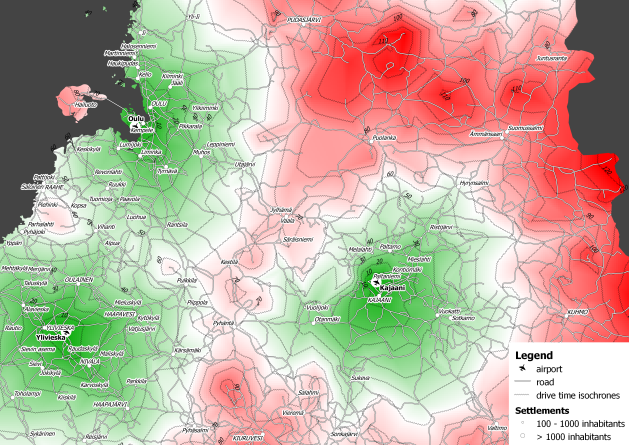
Drive Time Isochrones – An Example Using Finnish Airports

Site analyses can benefit greatly from using “drive-time” isochrones to define the study area. Drive time isochrones are often significantly different from simple buffer areas which disregard natural barriers such as rivers or slow roads.

Of course, creating drive time isochrones requires more input data and more compute-intensive algorithms than a simple buffer analysis. It is necessary to create a routable network graph with adequate weights to be used by the routing algorithm.

One of the most popular routing  applications in the open source world is pgRouting for PostGIS enabled databases. I’ve already shown how to create drive time isochrones for one network node based on pgRouting and QGIS.  Today, I’ll show how to create drive time isochrones for a set of points – in this case all airports in Finland.

The first step is to find the closest network node to every airport:

ALTER TABLE airport
   ADD COLUMN nearest_node integer;

CREATE TABLE temp AS
   SELECT a.gid, b.id, min(a.dist)
   FROM
     (SELECT airport.gid,
             min(distance(airport.the_geom, node.the_geom)) AS dist
      FROM airport, node
      GROUP BY airport.gid) AS a,
     (SELECT airport.gid, node.id,
             distance(airport.the_geom, node.the_geom) AS dist
      FROM airport, node) AS b
   WHERE a.dist = b. dist
         AND a.gid = b.gid
   GROUP BY a.gid, b.id;

UPDATE airport
SET nearest_node =
   (SELECT id
    FROM temp
    WHERE temp.gid = airport.gid);

Then, we can calculate drive times between network nodes and “airport nodes”. I am still looking for the most efficient way to perform this calculation. The trivial solution I used for this example was to calculate all drive time values separately for each airport node (as described in “Creating Catchment Areas with pgRouting and QGIS”). Afterwards, I combined the values to find the minimum drive time for each network node:

CREATE table catchment_airport_final AS
SELECT id, the_geom, min (cost) AS cost
FROM catchment_airport
GROUP By id, the_geom;

The resulting point layer was imported into QGIS. Using TIN interpolation (from Interpolation plugin), you can calculate a continuous cost surface. And Contour function (from GDALTools) finally yields drive time isochrones.

Drive time isochrones around airports in northern Finland

Based on this analysis, it is possible to determine how many inhabitants live within one hour driving distance from an airport or how many people have to drive longer than e.g. ninety minutes to reach any airport.


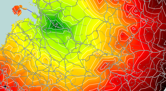
Creating Catchment Areas with pgRouting and QGIS

Based on the network created in my last post, I’ll now describe how to calculate the catchment area of a network node.

We need both network and node table. The cost attribute in my network table is called traveltime. (I used different speed values based on road category to calculate traveltime for road segments.) The result will be a new table containing all nodes and an additional cost attribute. And this is the query that calculates the catchment area around node #5657:

create table catchment_5657 as
select
    id,
    the_geom,
    (select sum(cost) from (
	   SELECT * FROM shortest_path('
	   SELECT gid AS id,
		  start_id::int4 AS source,
		  end_id::int4 AS target,
		  traveltime::float8 AS cost
	   FROM network',
	   5657,
	   id,
	   false,
	   false)) as foo ) as cost
from node

Then, I loaded the point table into QGIS and calculated a TIN based on the cost attribute. With “Contour” from GdalTools, you can visualize equal-cost areas even better:

Catchment area around node #5657 with contour lines

Between contour lines, there is a difference of 10 minutes travel time.


A Beginner’s Guide to pgRouting

The aim of this post is to describe the steps necessary to calculate routes with pgRouting. In the end, we’ll visualize the results in QGIS.

This guide assumes that you have the following installed and running:

  • Postgres with PostGIS and pgAdmin
  • QGIS with PostGIS Manager and RT Sql Layer plugins

Installing pgRouting

pgRouting can be downloaded from www.pgrouting.org.

Building from source is covered by pgRouting documentation. If you’re using Windows, download the binaries and copy the .dlls into PostGIS’ lib folder, e.g. C:\Program Files (x86)\PostgreSQL\8.4\lib.

Start pgAdmin and create a new database based on your PostGIS template. (I called mine ‘routing_template’.) Open a Query dialog, load and execute the three .sql files located in your pgRouting download (routing_core.sql, routing_core_wrappers.sql, routing_topology.sql). Congratulations, you now have a pgRouting-enabled database.

Creating a routable road network

The following description is based on the free road network published by National Land Survey of Finland (NLS). All you get is one Shapefile containing line geometries, a road type attribute and further attributes unrelated to routing.

pgRouting requires each road entry to have a start and an end node id. We’ll create those now:

First step is to load roads.shp into PostGIS. This is easy using PostGIS Manager – Data – Load Data from Shapefile.

Next, we create start and end point geometries. I used a view:

CREATE OR REPLACE VIEW road_ext AS
   SELECT *, startpoint(the_geom), endpoint(the_geom)
   FROM road;

Now, we create a table containing all the unique network nodes (start and end points) and we’ll also give them an id:

CREATE TABLE node AS
   SELECT row_number() OVER (ORDER BY foo.p)::integer AS id,
          foo.p AS the_geom
   FROM (
      SELECT DISTINCT road_ext.startpoint AS p FROM road_ext
      UNION
      SELECT DISTINCT road_ext.endpoint AS p FROM road_ext
   ) foo
   GROUP BY foo.p;

Finally, we can combine our road_ext view and node table to create the routable network table:

CREATE TABLE network AS
   SELECT a.*, b.id as start_id, c.id as end_id
   FROM road_ext AS a
      JOIN node AS b ON a.startpoint = b.the_geom
      JOIN node AS c ON a.endpoint = c.the_geom

(This can take a while.)

I recommend adding a spatial index to the resulting table.

Calculating shortest routes

Let’s try pgRouting’s Shortest Path Dijkstra method. The following query returns the route from node #1 to node #5110:

SELECT * FROM shortest_path('
   SELECT gid AS id,
          start_id::int4 AS source,
          end_id::int4 AS target,
          shape_leng::float8 AS cost
   FROM network',
1,
5110,
false,
false)

Final step: Visualization

With RT Sql Layer plugin, we can visualize the results of a query. The results will be loaded as a new layer. The query has to contain both geometry and a unique id. Therefore, we’ll join the results of the previous query with the network table containing the necessary geometries.

SELECT *
   FROM network
   JOIN
   (SELECT * FROM shortest_path('
      SELECT gid AS id,
          start_id::int4 AS source,
          end_id::int4 AS target,
          shape_leng::float8 AS cost
      FROM network',
      1,
      5110,
      false,
      false)) AS route
   ON
   network.gid = route.edge_id

In my case, this is how the result looks like:
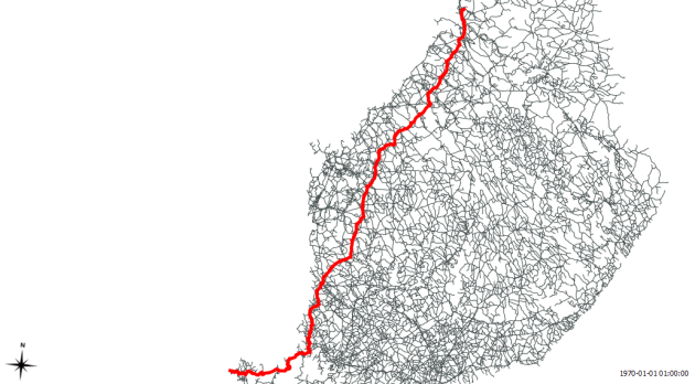
Route from node #1 to node #5110


Smaller Toolbar Icons for QGIS

Do you have a small resolution screen and want to use QGIS? Then you know the problem of toolbars using up precious screen estate.

In QGIS 1.7

You find the option to make icons smaller (16×16) or bigger (32×32) in the options dialog:

Options dialog with icon size option

If you are running a version of QGIS < 1.7

You can change the size of toolbar icons to any value you like – smaller or bigger than by default. And this is how it’s done (in Python console):

from PyQt4.QtGui import QToolBar
from PyQt4.QtCore import QSize

toolbars = qgis.utils.iface.mainWindow().findChildren(QToolBar)
for toolbar in toolbars:
    toolbar.setIconSize(QSize(16,16))

All toolbar icons will be scaled down to 16×16 pixels.

Kudos to Webrian on forum.qgis.org for this tip and to Nathan for pointing out how to access all toolbars.


Printing Web Maps with QGIS Mapserver

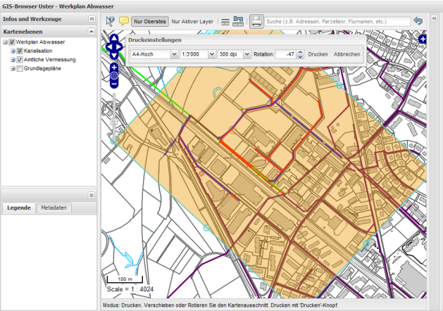
Great news: Sourcepole has extended QGIS server to offer printing functionality for web maps based on print composer.

Screenshot - Selecting a print extent

Selecting a print extent

You can test this functionality yourself on gis.uster.ch/webgis. The viewers are GeoExt-based. User can intuitively select a layout, extent, scale, rotation and resolution for printing. QGIS server will return a printable PDF.

If you want to learn more about what goes on behind the scenes, you find a good description on Sourcepole’s website.


How to Add a Legend to Your PyQGIS Application

In his post “Layer list widget for PyQGIS applications”, German Carrillo describes how to add a legend to your own PyQGIS application. You get to download the source code for the legend widget to include into your project.


QGIS with WPS Plugin in Action

The following video by soerengebbert shows the latest developments in OS WPS applications: PyWPS (using wps-grass-bridge to integrate GRASS modules as WPS processes), GRASS 7, and QGIS using the qwps plugin by Horst Düster (all latest svn versions).


  • <<
  • Page 14 of 15 ( 292 posts )
  • >>
  • gis

Back to Top

Sustaining Members