What's Changed

• Fix toggling of geometry editor type using the stylus
• Fix additional camera crashes

What's Changed

• Fix SSL-enabled postgis layer crash

Trajectools development started back in 2018 but has been on hold since 2020 when I realized that it would be necessary to first develop a solid trajectory analysis library. With the MovingPandas library in place, I’ve now started to reboot Trajectools.

Trajectools v2 builds on MovingPandas and exposes its trajectory analysis algorithms in the QGIS Processing Toolbox. So far, I have integrated the basic steps of

1. Building trajectories including speed and direction information from timestamped points and
2. Splitting trajectories at observation gaps, stops, or regular time intervals.

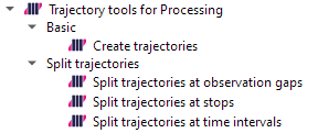
The algorithms create two output layers:

• Trajectory points with speed and direction information that are styled using arrow markers
• Trajectories as LineStringMs which makes it straightforward to count the number of trajectories and to visualize where one trajectory ends and another starts.

So far, the default style for the trajectory points is hard-coded to apply the Turbo color ramp on the speed column with values from 0 to 50 (since I’m simply loading a ready-made QML). By default, the speed is calculated as km/h but that can be customized:

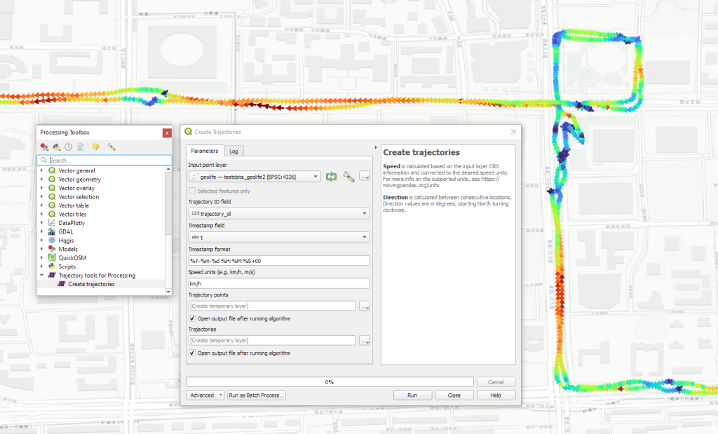
I don’t have a solution yet to automatically create a style for the trajectory lines layer. Ideally, the style should be a categorized renderer that assigns random colors based on the trajectory id column. But in this case, it’s not enough to just load a QML.

In the meantime, I might instead include an Interpolated Line style. What do you think?

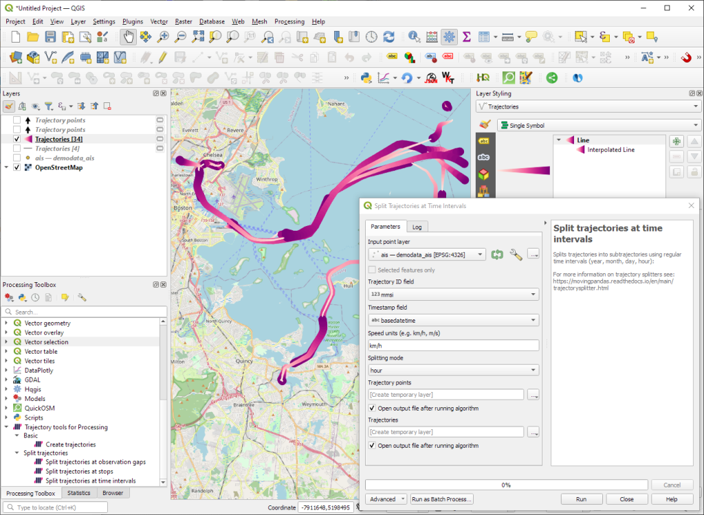
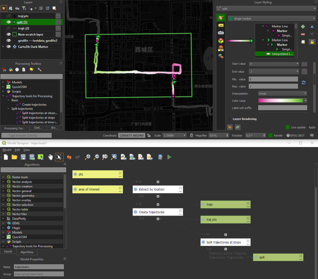
Of course, the goal is to make Trajectools interoperable with as many existing QGIS Processing Toolbox algorithms as possible to enable efficient Mobility Data Science workflows.

The easiest way to set up QGIS with MovingPandas Python environment is to install both from conda. You can find the instructions together with the latest Trajectools development version at: https://github.com/movingpandas/qgis-processing-trajectory

This post is part of a series. Read more about movement data in GIS.

Changes

🚀 Features

• QField can now snap to common angles when digitizing lines and polygons
• Expression-driven locking of geometry per feature
• QField's QML camera now adds direction metadata alongside geographical information
• QField's QML also features a grid overlay
• Vertex editor has again a new undo mechanism and capability to select a vertex by finger tapping on the screen
• @positioning_orientation variable available when running on devices equipped with a compass
• Functionality to allow for non-cloud projects to be updated through a ZIP file containing refreshed and/or new datasets and project file

✨ Improvements

• Improvement on the rendering of the coordinate cursor and digitizing rubber bands to insure visibility against both light and dark backgrounds
• Screen lock improvements, including disabling interactions with the back button
• Significant stability improvements; in particular, a bad camera-related crash in the upstream Qt library has been resolved
• Better handling of camera, microphone, and location permissions

The launch of QField 3.0 was a big deal, but now we’re back to focusing on smaller, more frequent updates. Don’t let the shorter change log for 3.1 trick you – there are lots of cool new features in this update!

Main highlights

One of the main improvements in this release is the brand-new functionality to enable snapping to common angles while digitizing. When enabled, the coordinate cursor will snap to configured angles alongside a visual guideline. This comes in handy when adding new geometries while surveying features with regular angles (e.g. buildings, parking lots, etc.). As QField gets more digitizing functionalities, we’ve taken the time to implement a nifty UI that collapses digitizing toggle buttons into a drawer, leaving extra space for the map canvas to shine through.

In addition, the vertex editor – one of QField’s most advanced geometry tools – received tons of love during this development cycle, focusing on improving its usability. Changes worth mentioning include:

• A new undo button allows users to revert individual vertex manipulations in case of mistaken adjustment, which can save you from having to cancel a large set of ongoing manipulations;
• The possibility to select vertices using finger tapping on the screen, dramatically improving the user experience;
• Clearer on-screen markers to represent vertices and
• Tons of bug fixes to the vertex editor itself, as well as the broader set of geometry tools.

It is now possible to lock the geometry of individual features within a single vector layer. While QField has long supported the concept of a locked geometry state for vector layers, that was until now a layer-wide toggle. With the new version of QField, a data-defined property can dictate whether a given feature geometry can be edited. Interested in geofenced geometry editing? We’ve got you covered This functionality requires the latest version of QFieldSync, which is available through QGIS’ plugin manager.

Noticeably improvements

Permission handling has been improved across all platforms. On Android, QField now delays the permission request for camera, microphone, location, and Bluetooth access until needed. This makes for a much friendlier user experience.

QField 3.0 was one of the largest releases, with major changes in its underlying libraries, including a migration to Qt 6. With the community’s help, we have spent countless hours testing before release. However, it is never a bulletproof process, and that version came with a few noticeable regressions. In particular, camera handling on Android suffered from upstream issues with Qt. We’ve tracked as many of those as possible, making this new version much more stable. One lingering camera issue remains and will be fixed upstream in the next three weeks; we’ll update as soon as it is available.

Finally, long-time users of QField will notice improvements in how geometry highlights and digitizing rubber bands are drawn. We’ve doubled down on efforts to ensure that the digitized geometries and the coordinate cursor itself are always clearly visible, whether overlaid against the canvas’s light or dark parts.

We want to extend a heartfelt thank you to our sponsors for their generous support. If you’re inspired by the developments in QField and want to contribute, please consider donating. Your support will help us continue to innovate and improve this tool for everyone’s benefit.

The GRASS GIS Annual Report for 2023 highlights a year of significant achievements and developments in the GRASS GIS project, which celebrated its 40th anniversary. Here’s a summary of the report: Community Meeting: The GRASS GIS Community Meeting was held in June at the Czech Technical University in Prague, bringing together a diverse group of […]

The post GRASS GIS Annual Report 2023 appeared first on Markus Neteler Consulting.

Dear QGIS Community,

We recently held our 2023 QGIS Annual General Meeting. The minutes of this meeting are available for all to view.

This year, we did not have PSC elections. Anita Graser will continue as Vice-Chair, I will continue to serve on the PSC as chair, and our longstanding treasurer, Andreas Neumann, will complete the board. Furthermore, Jürgen Fischer, Alessandro Pasotti, and Régis Haubourg will continue on the PSC. Last but certainly not least, the PSC is completed by our project founder, Gary Sherman, and long-term PSC member Tim Sutton, who serve on the PSC as honorary PSC members. They both set the standard for our excellent project culture, and it is great to have his continued presence.

QGIS has been growing from strength to strength, backed by a fantastic community of kind and collaborative users, developers, contributors and funders. This year, we reached another important milestone for the project’s sustainability by welcoming our first flagship sustaining member – Felt. I look forward to seeing how it continues to grow and flourish.

Rock on QGIS!

Cheers

Marco Bernasocchi (QGIS.ORG Chair)

Sorry, mostly interested for dutch readers

Very simple way of how to display map service in QGI3 without a map server.

New version of MapTiler QGIS Plugin 3.0 with detailed global terrain, contour lines, hillshading, and maps using these terrain data for outdoor activities.

The new version of the MapTiler plugin pushes our maps from MapTiler Cloud almost to perfection

Open-source plugin for QGIS that loads fast vector maps. Change colors and fonts of the map to get unique look.

Details of MapTiler QGIS Plugin 3.0 with a global terrain basemap and customizable OpenStreetMap vector tiles.

The new QGIS 3.14 version adds support for the native loading of vector tiles. The easiest way to load them is via the recently released plugin.

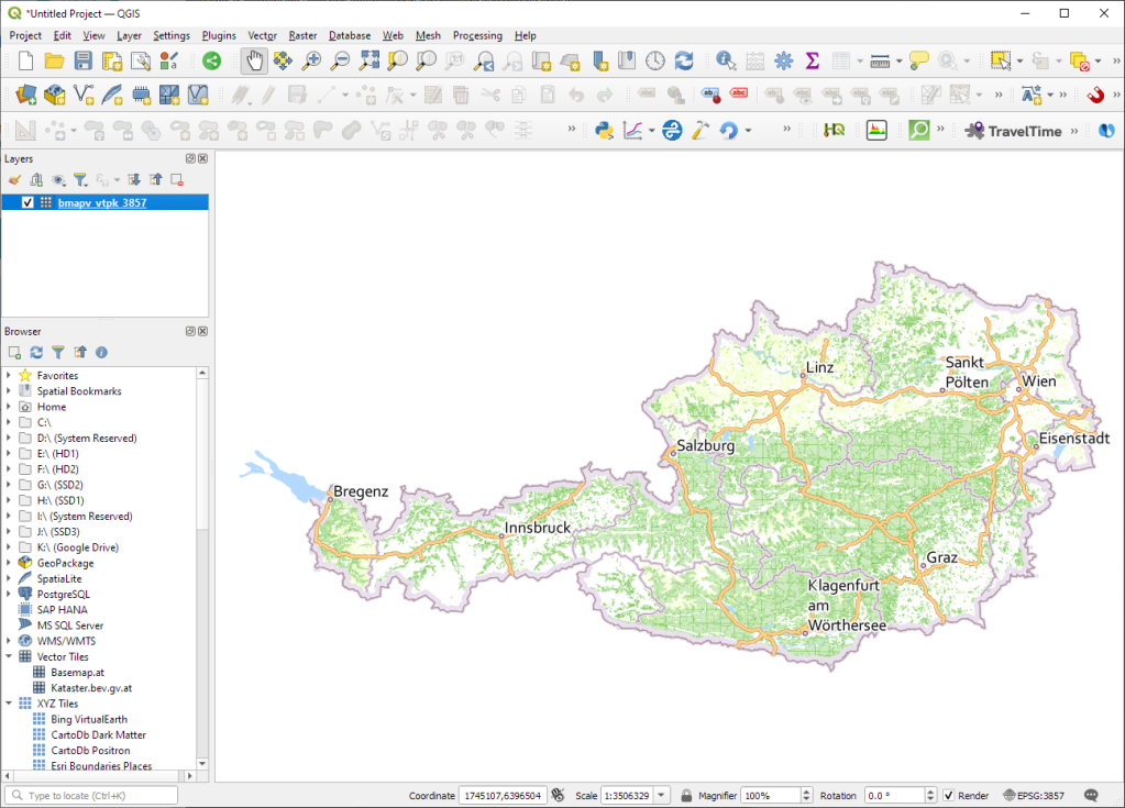
Starting from 3.26, QGIS now supports .vtpk (Vector Tile Package) files out of the box! From the changelog:

ESRI vector tile packages (VTPK files) can now be opened directly as vector tile layers via drag and drop, including support for style translation.

This is great news, particularly for users from Austria, since this makes it possible to use the open government basemap.at vector tiles directly, without any fuss:

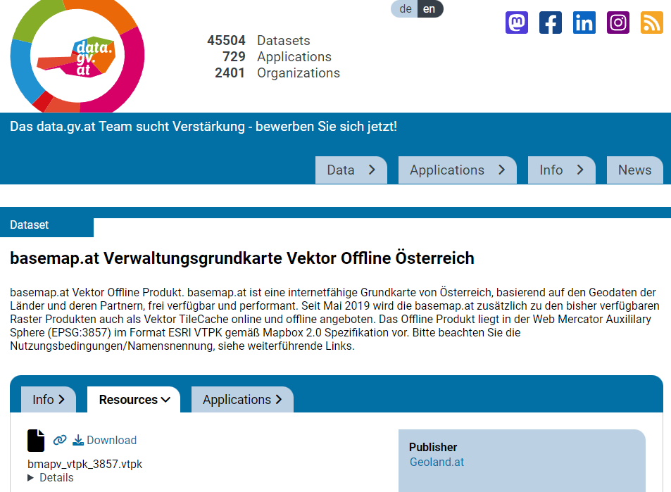
1. Download the 2GB offline vector basemap from https://www.data.gv.at/katalog/de/dataset/basemap-at-verwaltungsgrundkarte-vektor-offline-osterreich

2. Add the .vtpk as a layer using the Data Source Manager or via drag-and-drop from the file explorer

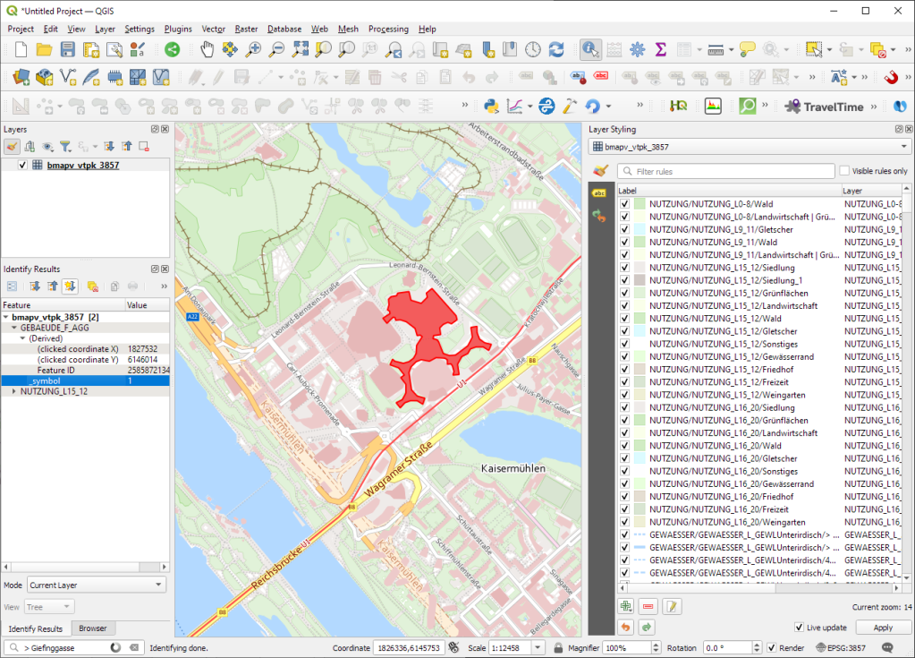
3. All done and ready, including the basemap styling and labeling — which we can customize as well:

Kudos to https://wien.rocks/@DieterKomendera/111568809248327077 for bringing this new feature to my attention.

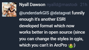
PS: And interesting tidbit from the developer of this feature, Nyall Dawson:

Today, I want to point out a blog post over at

https://geocompx.org/post/2023/geocompy-bp1/

In this post, Jakub Nowosad introduces our book “Geocomputation with Python”, also known as geocompy. It is an open-source book on geographic data analysis with Python, written by Michael Dorman, Jakub Nowosad, Robin Lovelace, and me with contributions from others. You can find it online at https://py.geocompx.org/

Changes

🐛 Bug Fixes

• Fix crash when using external GNSS devices, a regression caused by the permission handling changes.

Changes

✨ Improvements

• Update Sentry SDK to increase app stability.

Changes

✨ Improvements

• Harmonized and improved feature form drawer width when adding new features

Previously, we mapped neo4j spatial nodes. This time, we want to take it one step further and map relationships.

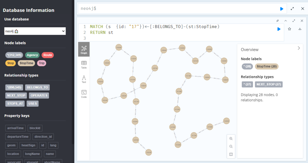
A prime example, are the relationships between GTFS StopTime and Trip nodes. For example, this is the Cypher query to get all StopTime nodes of Trip 17:

MATCH 
    (t:Trip  {id: "17"})
    <-[:BELONGS_TO]-
    (st:StopTime) 
RETURN st

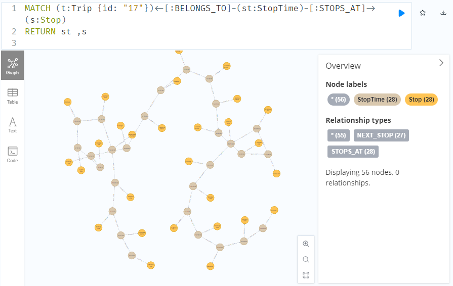
To get the stop locations, we also need to get the stop nodes:

MATCH 
    (t:Trip {id: "17"})
    <-[:BELONGS_TO]-
    (st:StopTime)
    -[:STOPS_AT]->
    (s:Stop)
RETURN st ,s

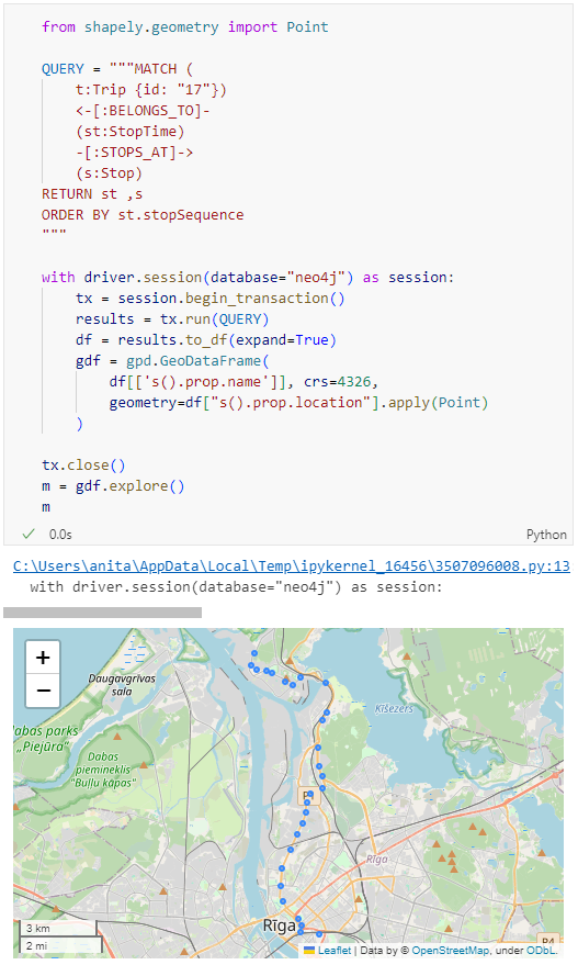
Adapting our code from the previous post, we can plot the stops:

from shapely.geometry import Point

QUERY = """MATCH (
    t:Trip {id: "17"})
    <-[:BELONGS_TO]-
    (st:StopTime)
    -[:STOPS_AT]->
    (s:Stop)
RETURN st ,s
ORDER BY st.stopSequence
"""

with driver.session(database="neo4j") as session:
    tx = session.begin_transaction()
    results = tx.run(QUERY)
    df = results.to_df(expand=True)
    gdf = gpd.GeoDataFrame(
        df[['s().prop.name']], crs=4326,
        geometry=df["s().prop.location"].apply(Point)
    )

tx.close() 
m = gdf.explore()
m

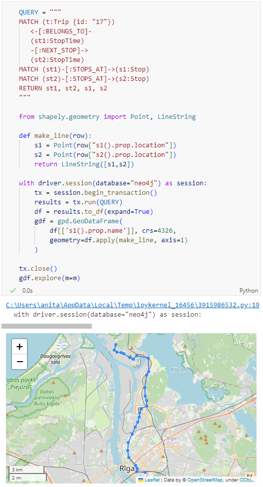
Ordering by stop sequence is actually completely optional. Technically, we could use the sorted GeoDataFrame, and aggregate all the points into a linestring to plot the route. But I want to try something different: we’ll use the NEXT_STOP relationships to get a DataFrame of the start and end stops for each segment:

QUERY = """
MATCH (t:Trip {id: "17"})
   <-[:BELONGS_TO]-
   (st1:StopTime)
   -[:NEXT_STOP]->
   (st2:StopTime)
MATCH (st1)-[:STOPS_AT]->(s1:Stop)
MATCH (st2)-[:STOPS_AT]->(s2:Stop)
RETURN st1, st2, s1, s2
"""

from shapely.geometry import Point, LineString

def make_line(row):
    s1 = Point(row["s1().prop.location"])
    s2 = Point(row["s2().prop.location"])
    return LineString([s1,s2])

with driver.session(database="neo4j") as session:
    tx = session.begin_transaction()
    results = tx.run(QUERY)
    df = results.to_df(expand=True)
    gdf = gpd.GeoDataFrame(
        df[['s1().prop.name']], crs=4326,
        geometry=df.apply(make_line, axis=1)
    )

tx.close() 
gdf.explore(m=m)

Finally, we can also use Cypher to calculate the travel time between two stops:

MATCH (t:Trip {id: "17"})
   <-[:BELONGS_TO]-
   (st1:StopTime)
   -[:NEXT_STOP]->
   (st2:StopTime)
MATCH (st1)-[:STOPS_AT]->(s1:Stop)
MATCH (st2)-[:STOPS_AT]->(s2:Stop)
RETURN st1.departureTime AS time1, 
   st2.arrivalTime AS time2, 
   s1.location AS geom1, 
   s2.location AS geom2, 
   duration.inSeconds(
      time(st1.departureTime), 
      time(st2.arrivalTime)
   ).seconds AS traveltime

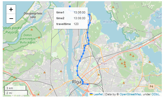
As always, here’s the notebook: https://github.com/anitagraser/QGIS-resources/blob/master/qgis3/notebooks/neo4j.ipynb