Related Plugins and Tags

QGIS Planet

Scalable spatial vector data processing

Working with movement data analysis, I’ve banged my head against performance issues every once in a while. For example, PostgreSQL – and therefore PostGIS – run queries in a single thread of execution. This is now changing, with more and more functionality being parallelized. PostgreSQL version 9.6 (released on 2016-09-29) included important steps towards parallelization, including parallel execution of sequential scans, joins and aggregates. Still, there is no parallel processing in PostGIS so far (but it is under development as described by Paul Ramsey in his posts “Parallel PostGIS II” and “PostGIS Scaling” from late 2017).

At the FOSS4G2016 in Bonn, I had the pleasure to chat with Shoaib Burq who ran the “An intro to Apache PySpark for Big Data GeoAnalysis” workshop. Back home, I downloaded the workshop material and gave it a try but since I wanted a scalable system for storing, analyzing, and visualizing spatial data, it didn’t really seem to fit the bill.

Around one year ago, my search grew more serious since we needed a solution that would support our research group’s new projects where we expected to work with billions of location records (timestamped points and associated attributes). I was happy to find that the fine folks at LocationTech have some very promising open source projects focusing on big spatial data, most notably GeoMesa and GeoWave. Both tools take care of storing and querying big spatio-temporal datasets and integrate into GeoServer for publication and visualization. (A good – if already slightly outdated – comparison of the two has been published by Azavea.)

My understanding at the time was that GeoMesa had a stronger vector data focus while GeoWave was more focused on raster data. This lead me to try out GeoMesa. I published my first steps in “Getting started with GeoMesa using Geodocker” but things only really started to take off once I joined the developer chats and was pointed towards CCRI’s cloud-local “a collection of bash scripts to set up a single-node cloud on your desktop, laptop, or NUC”. This enabled me to skip most of the setup pains and go straight to testing GeoMesa’s functionality.

The learning curve is rather significant: numerous big data stack components (including HDFS, Accumulo, and GeoMesa), a most likely new language (Scala), as well as the Spark computing system require some getting used to. One thing that softened the blow is the fact that writing queries in SparkSQL + GeoMesa is pretty close to writing PostGIS queries. It’s also rather impressive to browse hundreds of millions of points by connecting QGIS TimeManager to a GeoServer WMS-T with GeoMesa backend.

Spatial big data stack with GeoMesa

One of the first big datasets I’ve tested are taxi floating car data (FCD). At one million records per day, the three years in the following example amount to a total of around one billion timestamped points. A query for travel times between arbitrary start and destination locations took a couple of seconds:

Travel time statistics with GeoMesa (left) compared to Google Maps predictions (right)

Besides travel time predictions, I’m also looking into the potential for predicting future movement. After all, it seems not unreasonable to assume that an object would move in a similar fashion as other similar objects did in the past.

Early results of a proof of concept for GeoMesa based movement prediction

Big spatial data – both vector and raster – are an exciting challenge bringing new tools and approaches to our ever expanding spatial toolset. Development of components in open source big data stacks is rapid – not unlike the development speed of QGIS. This can make it challenging to keep up but it also holds promises for continuous improvements and quick turn-around times.

If you are using GeoMesa to work with spatio-temporal data, I’d love to hear about your experiences.

AmsterdamTimeMachine

Via twitter: AmsterdamTimeMachine.nl. Jan Hartman’s and WebMappers hard work of georeferencing a set of Old Amsterdam maps: http://amsterdamtimemachine.nl. 6 XYZ-Map services with maps old as 1625 to have a look into history, off course also to be loaded in QGIS Wanna see ‘the red light district’ in 1625? Or see Dutch 17th century glory on … Continue reading AmsterdamTimeMachine

Coding a QgsLocator (Plugin)

What is a Locator (plugin) Some months ago, Nyall Dawson silently dropped a nice widget into the lower left corner of your QGIS screen: People familiar with QtCreator (the Qt-development environment) should recognize it as a QtCreator Locator look-a-like: a way to (very) quickly search in your project for words, classes, bookmarks, help topics, files … Continue reading Coding a QgsLocator (Plugin)

Movement data in GIS #13: Timestamp labels for trajectories

In Movement data in GIS #2: visualization I mentioned that it should be possible to label trajectory segments without having to break the original trajectory feature. While it’s not a straightforward process, it is indeed possible to create timestamp labels at desired intervals:

The main point here is that we cannot use regular labels because there would be only one label for the whole trajectory feature. Instead, we are using a marker line with a font marker:

By default, font markers only display one character from a given font but by using expressions we can make it display longer text, including datetime strings:

If you want to have a label at every node of the trajectory, the expression looks like this:

format_date( 
   to_datetime('1970-01-01T00:00:00Z')+to_interval(
      m(start_point(geometry_n(
         segments_to_lines( $geometry ),
         @geometry_part_num)
      ))||' seconds'
   ),
   'HH:mm:ss'
)

You probably remember those parts of the expression that extract the m value from previous posts. Note that – compared to 2016 – it is now necessary to add the segments_to_lines() function.

The m value (which stores time as seconds since Unix epoch) is then converted to datetime and finally formatted to only show time. Of course you can edit the datetime format string to also include the date.

If we only want a label every 30 seconds, we can add a case statement around that:

CASE WHEN 
m(start_point(geometry_n(
   segments_to_lines( $geometry ),
   @geometry_part_num)
)) % 30 = 0
THEN
format_date( 
   to_datetime('1970-01-01T00:00:00Z')+to_interval(
      m(start_point(geometry_n(
         segments_to_lines( $geometry ),
         @geometry_part_num)
      ))||' seconds'
   ),
   'HH:mm:ss'
)
END

This works well if the trajectory sampling interval is fairly regular. This is not always the case and that means that the above case statement wouldn’t find many nodes with a timestamp that ends in :30 or :00. In such a case, we could resort to labeling nodes based on their order in the linestring:

CASE WHEN 
 @geometry_part_num  % 30 = 0
THEN
...

Thanks a lot to @JuergenEFischer for providing a solution for converting seconds since Unix epoch to datetime without a custom function!

Note that expressions using @geometry_part_num currently suffer from the following issue: Combination of segments_to_lines($geometry) and @geometry_part_num gives wrong segment numbers


This post is part of a series. Read more about movement data in GIS.

Reports from the winning grant proposals 2017

While we are waiting for this year’s grant proposals to come in, it is time to look back at last year’s winning proposals and their results. These are the reports on the work that has been done within the individual projects:

QGIS 3D – Martin Dobias

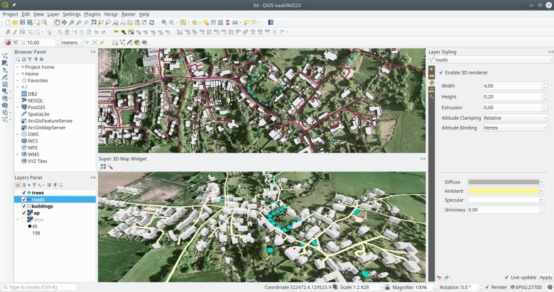
Results are included in the QGIS 3.0 release. As proposed in the grant, a new 3D map view has been added together with GUI for easy configuration of 3D rendering. The 3D view displays terrain (either from a DEM raster layer or a simple flat area) with 2D map rendered on top of the terrain. In addition to that, vector layers can be rendered as true 3D entities: points may be visualized as simple geometric shapes or as 3D models (loaded from a file), polygons and linestrings are tessellated into 3D geometries. 2D polygons can be turned into 3D objects using extrusion, possibly with data-defined height – an easy way how to display buildings, for example. Data with 3D coordinates have the Z values in geometries respected. Although the 3D view is still in its early stages, it is already usable for many use cases. Hopefully this functionality will help to attract even more users to QGIS!

More details: https://github.com/qgis/QGIS-Enhancement-Proposals/issues/105

Improvements to relations – Régis Haubourg

Various improvements for deep relations with PostgreSQL were successfully added in QGIS 3.0:

Add consistency to UI controls – Nyall Dawson

We’ve unified all the various opacity, rotation and scale controls to use the same terminology and numeric scales. We’ve also updated ALL methods for setting opacity, rotation and scale within the PyQGIS API to use consistent naming and arguments, making the API more predictable and easy to use. Lastly, we’ve also added a new reusable opacity widget (QgsOpacityWidget) to the GUI library so that future code can (and 3rd party scripts and plugins) can follow the new UI conventions for opacity handling.

Extend unit test coverage for geometry classes – Nyall Dawson

We’ve extended the unit testing coverage for all the underlying geometry primitive classes (points, lines, polygons, curves, collections, etc) so that all these classes have as close to 100% unit test coverage as possible. In the process, we identified and fixed dozens of bugs in the geometry library, and naturally added additional unit tests to avoid regressions in future releases. As a result QGIS’ core geometry engine is much more stable. Furthermore, we utilised the additional test coverage to allow us to safely refactor some of the slower geometry operations, meaning that many geometry heavy operations will perform much faster in QGIS 3.0.

Processing algorithm documentation – Matteo Ghetta & Alexander Bruy

The new Help system is landed and already available: when opening a Processing algorithm and clicking on the Help button, the guide of the algorithm will be showed in the default browser.

Many of the QGIS Processing algorithm guides have been enhanced with pictures and new or enhanced descriptions. A consistency number of Pull Requests have been already merged and many others are in review. Just a few descriptions need to be still enhanced.

Currently all the QGIS algorithms have been described and all the PR in the doc repository have been merged (kudos to Harrissou for all the reviews!).

Right now the Help button of each Processing dialog will open the related page of the algorithm, BUT:

  • if the name of the algorithm is made by only ONE word (e.g. clip, intersection…), the help button will open the browser to also the correct section (that is, the user will see directly the description of the related algorithm)
  • if the name of the algorithm has >1 words (e.g. split polygon with lines, lines to polygon, ecc.) the Help button will open the correct page (so the algorithm GROUP) but is not able to go to the correct algorithm anchor. This is because sphinx converts “split with lines” in “split-with-lines” while QGIS system will always cast the words “split-with-lines” in “splitwithlines”. Not a big deal, but IMHO a pity.
    We are really too close to the solution.

So Processing Help system right now consists of:

  • QGIS algs -> documented
  • GDAL algs -> documented
  • GRASS -> documented (own docs)
  • Orfeo -> documented (own docs)
  • SAGA -> nothing documented

Thanks to QGIS Grants to provide this chance to give a big improvement to the Processing framework even if not in a coding way!


Last but not least, we had another project that was not part of the grant programme but was also funded by QGIS.ORG in 2017:

Python API documentation – Denis Rouzaud

QGIS Python API Documentation is created using Sphinx and this work is available on Github. The repo is a fork of QGIS’ one and has been merged in the meantime. The docs are available at qgis.org/pyqgis. It uses a new theme (sphinx_rtd_theme aka ReadTheDocs theme). Some improvements were brought in (not exhaustive):

  • QGIS theming with colors and icon
  • Foldable toctree
  • Summary of methods and attributes for classes
  • Module index (not available before)
  • Correct display of overloaded methods

Full Python signature in Docstring

In former SIP versions, it was not possible to use the auto generated signature if a Docstring already existed. This means any documented method could not have a signature created. Unfortunately for this project, the vast majority of methods in QGIS API are documented!

The source code of SIP was modified and theses changes got merged upstream. See rev 1788 to 1793 in SIP changelog. It will be released in upcoming 4.19.7 version. QGIS source code was modified accordingly to prepend auto generated Python signatures to existing Docstrings. Using a CMake configuration file for each module (core.sip.in, gui.sip.in, etc.) was required to avoid syntax errors when using former version of SIP (since bumping minimum version is not realistic).

Sipify adjustments

Many things were fixed in sipify script :

  • Creation of links to classes, methods
  • Handling/fixing of Doxygen annotations \see, \note, \param
  • Handling of code snippets: c++ vs Python. Only Python are shown.

Thank you to everyone who participated and made this round of grants a great success and thank you to all our sponsor and donors who make this initiative possible!

Anita

Drill down (cascading) forms in QGIS crowdfund – final stretch!

Update: donations are now closed, with the outcome of the campaign pending!

We’re nearing the final hours of our crowd funding campaign to implement a drill-down (cascading) field support within QGIS forms, and thanks to numerous generous backers we’re very close to hitting the funding goal! This is a really exciting new feature which would help add greater flexibility and power to QGIS feature forms, but in order to implement it for QGIS 3.2 we need to hit the funding target by 11 May 2018.

As a result, we’re dropping the minimum contribution amount and throwing open the campaign for payments of any amount. These smaller payment will be treated as direct donations to the campaign, so unlike the standard campaign backing these are payable up front. In the case that the campaign IS NOT successful, the donations will not be refunded and will instead be reinvested back into the QGIS (via bug fixing and maintenance efforts). Of course, if you’d prefer to pledge using the standard crowdfunding “no payment if campaign unsuccessful” model you’re more than welcome to! (Full details are available on the campaign page).

Donations closed – outcome pending!

Full details are available on the campaign page.

Docker images for QGIS

With support from Orange we’ve created Docker images for QGIS. All the material for building and running these images is open-source and freely available on GitHub: https://github.com/Oslandia/docker-qgis.
The docker-qgis repository includes two Docker images: qgis-build and qgis-exec.

The qgis-build image includes all the libraries and tools necessary for building QGIS from source. Building QGIS requires installing a lot of dependencies, so it might not be easy depending on the Operating System you use. The qgis-build image makes it easy and repeatable. The result of a QGIS build is Debian Stretch packages that can be used for building the qgis-exec image, as explained below.

The qgis-exec image includes a runtime environment for QGIS Server. The image makes it easy to deploy and run QGIS Server. It is meant to be be generic and usable in various contexts, and in production. There are two ways to build the qgis-exec image. It can be built from the official QGIS 3 Debian packages (http://qgis.org/debian/), or from local QGIS Debian Stretch packages that were built using the qgis-build image.

We encourage you to go test and use our images! We haven’t pushed the images to the Docker Hub yet, but this is in the plans.

Feel free to contact us on GitHub or by email for any question or request!

Preparing for the next LTR

Dear QGIS users,

As you know, QGIS 3 has recently been published. This version introduced big changes in  the code structure that, in addition to the new functionalities already exposed, makes our code base more modern and easier to expand and improve on in the future.

As a normal by-product of such a huge overhaul, these changes also triggered a series of new issues, that you, our users are helping to discover and document. Our objective is to eliminate the most important of these issues in time for what will be our next Long Term Release (LTR) – version 3.4. This release is scheduled for October 2018. The resources available from QGIS.ORG funds are limited, and we have already invested in QGIS 3.0 far more than we have done for any previous version.

Now is a great time for users, and particularly for power users, larger institutions and enterprises, to invest in QGIS bugfixing. You have a number of different options: donating your developers’ time or hiring a developer directly to resolve the bugs that annoy you most, sponsoring our foundation, or donating to QGIS.ORG.

Our targets are:

  • 20k€ within 2018-05-18 (for 3.2)
  • 40k€ within 2018-09-14 (for 3.4)

If you would like to help, feel free to contact us (preferably through the qgis-users or qgis-developers mailing list, or directly to [email protected]) for further details!

signature_qgis_cert

PDAL 1.7 packaged for Fedora including vertical datums and grids

Cologne city shown as colorized 3D point cloud (data source: openNRW Germany)In order to simplify the installation of the latest PDAL release (Point Data Abstraction Library, https://pdal.io/, version 1.7.0 1.7.2) on Fedora, I have created an updated set of RPM packages, again including the vertical datums and grids available from OSGeo (i.e., .gtx files from here).

The installation is as simple as this (the repository is located at Fedora’s COPR):

# enable extra repos to satisfy dependencies
sudo dnf copr enable neteler/pdal-hexer
sudo dnf copr enable neteler/points2grid
sudo dnf copr enable neteler/laszip

# install minimal dependencies
sudo dnf install hexer
sudo dnf install points2grid

# enable and install PDAL
sudo dnf copr enable neteler/pdal
sudo dnf install PDAL PDAL-vdatums

# run it
pdal-config --version
pdal --help

Enjoy!

The post PDAL 1.7 packaged for Fedora including vertical datums and grids appeared first on GFOSS Blog | GRASS GIS and OSGeo News.

PdokServicesPlugin, new version

This post is to announce the availability of a new version of the PdokServicePlugin. Unless a heavy user of Dutch Public Datasources (WMS, WFS, WCS), this is probably mostly interesting for Dutchies. But if you want to know how many kilometers somebody is living from the nearest Fire Department Station:

Movement data in GIS #12: why you should be using PostGIS trajectories

In short: both writing trajectory queries as well as executing them is considerably faster using PostGIS trajectories (as LinestringM) rather than the commonly used point-based approach.

Here are a couple of examples to give you an impression of the differences.

Spoiler alert! Trajectory queries are up to 500 times faster than comparable point-based queries.

A quick look at indexing

In both cases, we have indexed the tracker id, geometry, and time columns to speed up query processing.

The trajectory table has 3 indexes

  • gist (time_range)
  • gist (track gist_geometry_ops_nd)
  • btree (tracker)

The point-based table has 4 indexes

  • gist (pt)
  • btree (trajectory_id)
  • btree (tracker)
  • btree (t)

Length

First, let’s see how to determine trajectory length for all observed moving objects (identified by a tracker id).

Using the point-based approach, we first need to ensure that the points are in the correct temporal order, create the lines, and finally sum up their length:

WITH ordered AS (
 SELECT trajectory_id, tracker, t, pt
 FROM geolife.trajectory_pt
 ORDER BY t
), tmp AS (
 SELECT trajectory_id, tracker, st_makeline(pt) traj
 FROM ordered 
 GROUP BY trajectory_id, tracker
)
SELECT tracker, round(sum(ST_Length(traj::geography)))
FROM tmp
GROUP BY tracker 
ORDER BY tracker

With trajectories, we can go right to computing lengths:

SELECT tracker, round(sum(ST_Length(track::geography)))
FROM geolife.trajectory_ext
GROUP BY tracker
ORDER BY tracker

On my test system, the trajectory query run time is 22.7 sec instead of 43.0 sec for the point-based approach:

Duration

Compared to trajectory length, duration is less complicated in the point-based approach:

WITH tmp AS (
 SELECT trajectory_id, tracker, min(t) start_time, max(t) end_time
 FROM geolife.trajectory_pt
 GROUP BY trajectory_id, tracker
)
SELECT tracker, sum(end_time - start_time)
FROM tmp
GROUP BY tracker
ORDER BY tracker

Still, the trajectory query is less complex and much faster at 31 ms instead of 6.0 sec:

SELECT tracker, sum(upper(time_range) - lower(time_range))
FROM geolife.trajectory_ext
GROUP BY tracker
ORDER BY tracker

Temporal filter

Extracting trajectories that occurred during a certain time frame is another common use case:

WITH tmp AS (
 SELECT trajectory_id, tracker, min(t) start_time, max(t) end_time
 FROM geolife.trajectory_pt
 GROUP BY trajectory_id, tracker
)
SELECT trajectory_id, tracker, start_time, end_time
FROM tmp
WHERE end_time > '2008-11-26 11:00'
AND start_time < '2008-11-26 15:00'
ORDER BY tracker

This point-based query takes 6.0 sec while the shorter trajectory query finishes in 12 ms:

SELECT id, tracker, time_range
FROM geolife.trajectory_ext
WHERE time_range && '[2008-11-26 11:00+1,2008-11-26 15:00+01]'::tstzrange

or equally fast (12 ms) by making use of the n-dimensional index:

WHERE track &&&	ST_Collect(
 ST_MakePointM(-180, -90, extract(epoch from '2008-11-26 11:00'::timestamptz)),
 ST_MakePointM(180, 90, extract(epoch from '2008-11-26 15:00'::timestamptz))
)

Spatial filter

Finally, of course, let’s have a look at spatial filters, for example, trajectories that start in a certain area:

WITH my AS ( 
 SELECT ST_Buffer(ST_SetSRID(ST_MakePoint(116.31894,39.97472),4326),0.0005) areaA
), tmp AS (
 SELECT trajectory_id, tracker, min(t) t 
 FROM geolife.trajectory_pt
 GROUP BY trajectory_id, tracker
)
SELECT distinct traj.tracker, traj.trajectory_id 
FROM tmp
JOIN geolife.trajectory_pt traj
ON tmp.trajectory_id = traj.trajectory_id AND traj.t = tmp.t
JOIN my
ON ST_Within(traj.pt, my.areaA)

This point-based query takes 6.0 sec while the shorter trajectory query finishes in 488 ms:

WITH my AS ( 
 SELECT ST_Buffer(ST_SetSRID(ST_MakePoint(116.31894, 39.97472),4326),0.0005) areaA
)
SELECT id, tracker, ST_AsText(track)
FROM geolife.trajectory_ext
JOIN my
ON areaA && track
AND ST_Within(ST_StartPoint(track), areaA)

For more generic “does this trajectory intersect another geometry”, the points can also be aggregated to a linestring on the fly but that takes 21.9 sec:

I’ll be presenting more work on PostGIS trajectories at GI_Forum in Salzburg in July. In the talk, I’ll also have a look at the custom PG-Trajectory datatype. Here’s the full open-access paper:

Graser, A. (2018) Evaluating Spatio-temporal Data Models for Trajectories in PostGIS Databases. GI_Forum ‒ Journal of Geographic Information Science, 1-2018, 16-33. DOI: 10.1553/giscience2018_01_s16.

You can find my fork of the PG-Trajectory project – including all necessary fixes – on Bitbucket.


This post is part of a series. Read more about movement data in GIS.

Drill-down (cascading) forms in QGIS crowdfund launched!

We’ve just launched a new crowd funding campaign to implement a drill-down (cascading) field support within QGIS forms. Full details are available on the campaign page.

This is a really exciting new feature which would help add greater flexibility and power to QGIS feature forms! To make it possible we need 3500€ pledged before 11 May 2018. You can help make this a reality by supporting the campaign or by sharing the page and increasing exposure to the campaign. Updates to follow!

QGIS Grants #3: Call for Grant Proposals 2018

Dear QGIS Community

Our first two rounds of Grant Proposals were a great success. If you are an early adopter using QGIS 3.0, you can already try out some of the new capabilities that have arrived in QGIS thanks to these grants.

We are very pleased to announce the third round of grants is now available to QGIS contributors. The deadline for this round is Sunday, 13 May 2018. All the details for the grants are described in the application form, and for more context we encourage you to also read these articles:

We look forward to seeing all your great ideas about how to improve QGIS!

Anita Graser

QGIS PSC

QGIS Annual General Meeting – 2018

Dear QGIS Community


We recently held our 2018 QGIS Annual General Meeting. The minutes of this meeting are available for all to view. As I have previously announced, I have decided to step down as chair of the PSC this year, so this post is my last official act as QGIS Chair. Thank you all for the kind words and deeds of support you gave me during my time as project chair.

I would like to welcome our new QGIS Board Chair: Paolo Cavallini, and our new QGIS Board Vice-Chair and QGIS PSC Member, Marco Bernasocchi. In case you are not familiar with Paolo and Marco, you can find short introductions to them below. I am pleased also to say that the project governance is in good hands with Richard Duivenvoorde, Jürgen Fischer, Andreas Neumann and Anita Graser kindly making themselves available to serve on the PSC for another two years. It is also great to know that our project founder, Gary Sherman, continues to serve on the PSC as honorary PSC member. Gary set the standard for our great project culture and it is great to have his continued presence.

QGIS has been growing from strength to strength, backed by a really amazing community of kind and collaborative users, developers, contributors and funders. I am looking forward to seeing how it continues to grow and flourish and I am excited and confident it will do so with Paolo acting as the project chair and representative. Rock on QGIS!


Paolo Cavallini

Paolo

I got involved in QGIS long ago, first as a user, then more and more deeply in various activities, initiating and supporting various plugins and core functions (e.g. GDAL Tools, DB Manager), opening and managing bugs, taking care of GRASS modules, handling the trademark registration, etc. I acted as Finance and Marketing Advisor for several years. Currently, I manage the plugin approval process. Motivation: It’s such a pleasure building up, in a truly cooperative and democratic way, together with truly intelligent people, a tool that enables people to freely do their job or pursue their interests, that I cannot resist helping as much as I can.

Marco Bernasocchi (http://berna.io @mbernasocchi)

20180214_112925.jpg

I am an open source advocate, consultant, teacher and developer. My background is in geography with a specialization in geographic information science. I live in Switzerland in a small Romansh speaking mountain village where I love scrambling around the mountains to enjoy the feeling of freedom it gives me. I’m a very communicative person, I fluently speak Italian, German, French English and Spanish and love travelling. I work as director of OPENGIS.ch which I founded in 2011. Since 2015 I share the company ownership with Matthias Kuhn. At OPENGIS.ch LLC we (4 superstar devs and myself) develop, train and consult our client on any aspect related to QGIS. My first QGIS (to be correct for that time QuantumGIS) ever was “Simon (0.6)” during my BSc when the University of Zurich was teaching us proprietary products and I started looking around for Open Source alternatives. In 2008, when starting my MSc, I made the definitive switch to Ubuntu and I started working more and more with QGIS Metis (0.11) and ended developing some plugins and part of Globe as my Masters thesis. Since three years the University of Zurich invites me to hold two seminars on Entrepreneurship and Open Source. In November 2011 I attended my first Hackfest in Zürich where I started porting all QGIS dependencies and developing QGIS for Android under a Google Summer of Code. A couple of years and a lot of work later QField was born. Since then I’ve always tried to attend at least to one Hackfest per year to be able to feel first hand the strong bonds within our very welcoming community. In 2013 I was lucky enough to have a release named after a suggestion I saved you all from having QGIS 2.0 – Hönggerberg and giving you instead QGIS 2.0 – Dufour Beside my long story with QGIS as user and passionate advocate I have a long story as QGIS service provider where we are fully committed to its stability, feature richness and sustainable development. Furthermore, as WorldBank consultant, I am lucky enough to be sent now and then to spread the QGIS goodness in less fortunate countries. Motivation: One of my main motivation to be part of the PSC is to help QGIS keep this incredible growth rate by being even more attractive to new community members, sponsors and large/corporate users. To achieve this, the key is maintaining the right balance between sustainable processes (that guarantee the great quality QGIS has been known for) and an interesting and motivating grassroots project where community members can bloom and enjoy contributing in their most creative ways.


Regards

timsutton

Tim Sutton (outgoing Chair)

Optional parameters in QGIS Processing scripts & models

Remember the good old times when all parameters in Processing were mandatory?

Inputs and outputs are fixed, and optional parameters or outputs are not supported. [Graser & Olaya, 2015]

Since QGIS 2.14, this is no longer the case. Scripts, as well as models, can now have optional parameters. Here is how for QGIS 3:

When defining a Processing script parameter, the parameter’s constructor takes a boolean flag indicating whether the parameter should be optional. It’s false by default:

class qgis.core.QgsProcessingParameterNumber(
   name: str, description: str = '', 
   type: QgsProcessingParameterNumber.Type = QgsProcessingParameterNumber.Integer, 
   defaultValue: Any = None, 
   optional: bool = False,
   minValue: float = -DBL_MAX+1, maxValue: float = DBL_MAX)

(Source: http://python.qgis.org/api/core/Processing/QgsProcessingParameterNumber.html)

One standard tool that uses optional parameters is Add autoincremental field:

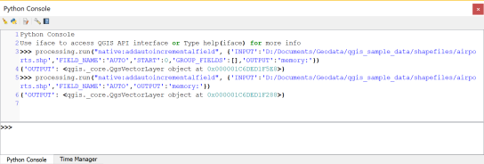
From Python, this algorithm can be called with or without the optional parameters:

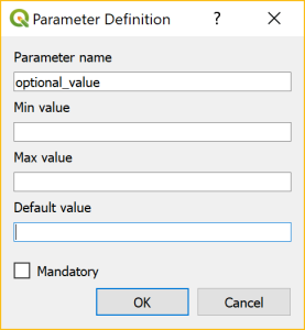
When building a model, an optional input can be assigned to the optional parameter. To create an optional input, make sure to deactivate the mandatory checkbox at the bottom of the input parameter definition:

Then this optional input can be used in an algorithm. For example, here the numerical input optional_value is passed to the Start values at parameter:

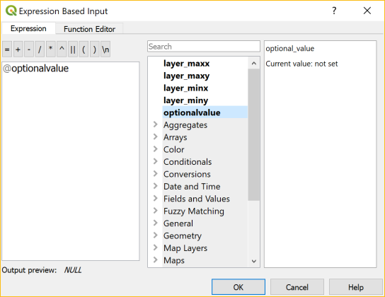
You can get access to all available inputs by clicking the … button next to the Start values at field. In this example, I have access to values of the input layer as well as  the optional value:

Once this is set up, this is how it looks when the model is run:

You can see that the optional value is indeed Not set.

References

Graser, A., & Olaya, V. (2015). Processing: A Python Framework for the Seamless Integration of Geoprocessing Tools in QGIS. ISPRS Int. J. Geo-Inf. 2015, 4, 2219-2245. doi:10.3390/ijgi4042219.

Processing script template for QGIS3

Processing has been overhauled significantly for QGIS 3.0. Besides speed-ups, one of the most obvious changes is the way to write Processing scripts. Instead of the old Processing-specific syntax, Processing scripts for QGIS3 are purely pythonic implementations of QgsProcessingAlgorithm.

Here’s a template that you can use to develop your own algorithms:

from qgis.PyQt.QtCore import QCoreApplication, QVariant
from qgis.core import (QgsField, QgsFeature, QgsFeatureSink, QgsFeatureRequest, QgsProcessing, QgsProcessingAlgorithm, QgsProcessingParameterFeatureSource, QgsProcessingParameterFeatureSink)
                      
class ExAlgo(QgsProcessingAlgorithm):
    INPUT = 'INPUT'
    OUTPUT = 'OUTPUT'

    def __init__(self):
        super().__init__()

    def name(self):
        return "exalgo"
    
    def tr(self, text):
        return QCoreApplication.translate("exalgo", text)
        
    def displayName(self):
        return self.tr("Example script")

    def group(self):
        return self.tr("Examples")

    def groupId(self):
        return "examples"

    def shortHelpString(self):
        return self.tr("Example script without logic")

    def helpUrl(self):
        return "https://qgis.org"
        
    def createInstance(self):
        return type(self)()
  
    def initAlgorithm(self, config=None):
        self.addParameter(QgsProcessingParameterFeatureSource(
            self.INPUT,
            self.tr("Input layer"),
            [QgsProcessing.TypeVectorAnyGeometry]))
        self.addParameter(QgsProcessingParameterFeatureSink(
            self.OUTPUT,
            self.tr("Output layer"),
            QgsProcessing.TypeVectorAnyGeometry))

    def processAlgorithm(self, parameters, context, feedback):
        source = self.parameterAsSource(parameters, self.INPUT, context)
        (sink, dest_id) = self.parameterAsSink(parameters, self.OUTPUT, context,
                                               source.fields(), source.wkbType(), source.sourceCrs())

        features = source.getFeatures(QgsFeatureRequest())
        for feat in features:
            out_feat = QgsFeature()
            out_feat.setGeometry(feat.geometry())
            out_feat.setAttributes(feat.attributes())
            sink.addFeature(out_feat, QgsFeatureSink.FastInsert)

        return {self.OUTPUT: dest_id}

This script just copies the features of the input layer to the output layer without any modifications. Add your logic to the processAlgorithm() function to get started.

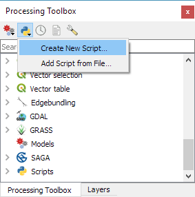
Use Create New Script from the Toolbox toolbar:

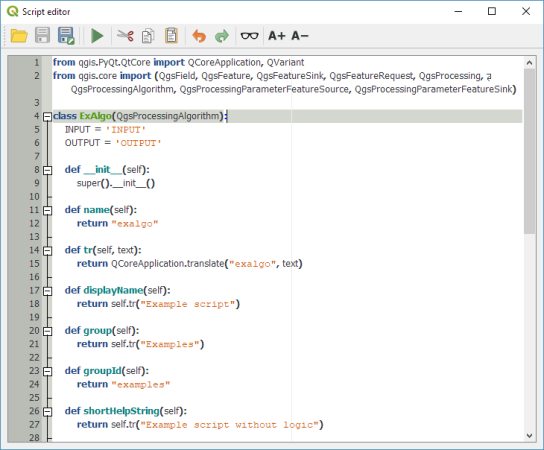
Paste the example script:

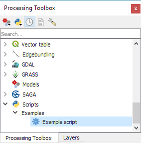
Once saved, the script will show up in the Processing toolbox:

Revisiting point & polygon joins

Joining polygon attributes to points based on their location is a very common GIS task. In QGIS 2, QGIS’ own implementation of “Join attributes by location” was much slower than SAGA’s “Add polygon attributes to points”. Thus, installations without SAGA were out of good options.

Luckily this issue (and many more) has been fixed by the rewrite of many geoprocessing algorithms for QGIS 3! Let’s revisit the comparison:

I’m using publicly available datasets from Naturalearth: The small scale populated places (243 points) and the large scale countries (255 polygons with many nodes). Turns out that QGIS 3’s built-in tool takes a little less than two seconds while the SAGA Processing tool requires a litte less than six seconds:

Like in the previous comparison, times were measured using the Python Console:

In both tools, only the countries’ SOVEREIGNT attribute is joined to the point attribute table:

import processing
t0 = datetime.datetime.now()
print("QGIS Join attributes by location ...")
processing.runAndLoadResults(
   "qgis:joinattributesbylocation", 
   {'INPUT':'E:/Geodata/NaturalEarth/vector_v4/natural_earth_vector/110m_cultural/ne_110m_populated_places.shp',
   'JOIN':'E:/Geodata/NaturalEarth/vector_v4/natural_earth_vector/10m_cultural/ne_10m_admin_0_countries.shp',
   'PREDICATE':[5],'JOIN_FIELDS':['SOVEREIGNT'],
   'METHOD':0,'DISCARD_NONMATCHING':False,'OUTPUT':'memory:'})
t1 = datetime.datetime.now()
print("Runtime: "+str(t1-t0))
print("SAGA Add polygon attributers to points ...")
processing.runAndLoadResults("saga:addpolygonattributestopoints", 
   {'INPUT':'E:/Geodata/NaturalEarth/vector_v4/natural_earth_vector/110m_cultural/ne_110m_populated_places.shp',
   'POLYGONS':'E:/Geodata/NaturalEarth/vector_v4/natural_earth_vector/10m_cultural/ne_10m_admin_0_countries.shp',
   'FIELDS':'SOVEREIGNT','OUTPUT':'C:/Users/anita/AppData/Local/Temp/processing_8b1bbde78de5490285dd530e115cca52/099660d88bf14c54a853cc230e388e55/OUTPUT.shp'})
t2 = datetime.datetime.now()
print("Runtime: "+str(t2-t1))

It is worth noting that it takes longer if more attributes are to be joined to the point layer attribute table. For example, if the JOIN_FIELDS parameter is empty:

'JOIN_FIELDS':[]

instead of

'JOIN_FIELDS':['SOVEREIGNT']

then the the Join attributes by location takes almost 16 seconds. (The country layer contains 71 attributes after all.)

(The SAGA tool currently allows only joining one attribute at a time.)

QGIS 3 Server deployment showcase with Python superpowers

Recently I was invited by the colleagues from OpenGIS.ch to lend a hand in a training session about QGIS server.

This was a good opportunity to update my presentation for QGIS3, to fix a few bugs and to explore the powerful capabilities of QGIS server and Python.

As a result, I published the full recipe of a Vagrant VM on github: https://github.com/elpaso/qgis3-server-vagrant

The presentation is online here: http://www.itopen.it/bulk/qgis3-server/

What’s worth mentioning is the sample plugins (I’ll eventually package and upload them to the official plugin site):


The VM uses 4 different (although similar) deployment strategies:

  • good old Apache + mod_fcgi and plain CGI
  • Nginx + Fast CGI
  • Nginx + standalone HTTP Python wrapped server
  • Nginx + standalone WSGI Python wrapped server

Have fun with QGIS server: it was completely refactored in QGIS 3 and it’s now better than ever!


The post QGIS 3 Server deployment showcase with Python superpowers first appeared on Open Web Solutions, GIS & Python Development.

(Nederlands) Je eerste 3-D kaart in QGIS 3.0

Sorry, this entry is only available in the Dutch language

Use your android phone’s GPS in QGIS

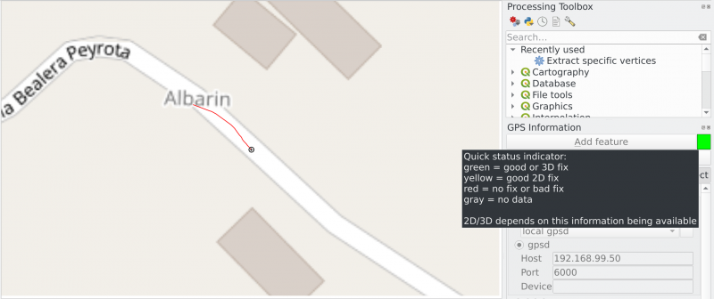
Do you want to share your GPS data from your phone to QGIS? Here is how:   QGIS comes with a core plugin named GPS Tools that can be enabled in the Plugin installer dialog:   There are several ways to forward data from your phone and most of them are very well described in the QGIS manual page: https://docs.qgis.org/testing/en/docs/user_manual/working_with_gps/plugins_gps.html What I’m going to describe here is mostly useful when your phone and your host machine running QGIS are on the same network (for example they are connected to the same WiFi access point) and it is based on the simple application GPS 2 NET   Once the application is installed and started on your phone, you need to know the IP address of the phone, on a linux box you can simply run a port scanner and it will find all devices connected to the port 6000 (the default port used by GPS 2 NET):  

# Assuming your subnet is 192.168.9

nmap -p 6000 192.168.1.*

Nmap scan report for android-8899989888d02271.homenet.telecomitalia.it (192.168.99.50)
Host is up (0.0093s latency).
PORT STATE SERVICE
6000/tcp open X11

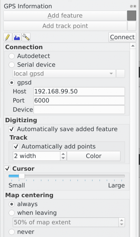
  Now, in QGIS you can open the plugin dialog through Vector -> GPS -> GPS Tools and enter the IP address and port of your GPS device:   Click on Connect button on the top right corner (mouse over the gray square for GPS status information)   Start digitizing!

The post Use your android phone’s GPS in QGIS first appeared on Open Web Solutions, GIS & Python Development.

  • <<
  • Page 48 of 141 ( 2819 posts )
  • >>

Back to Top

Sustaining Members