The forum (http://forum.qgis.org) has been closed for new registrations and marked read-only. Users have been encouraged to use http://gis.stackexchange.com instead.

If you have an thoughts on the closure, good, bad, or otherwise, please comment.

One thing I didn’t explain very well  in my other post was how to correctly set up value binding between your custom form and QGIS.  I didn’t explain it because at the time I didn’t know how.

The other day I was building a custom form QGIS for a project I am working on. I had named all the fields right, set the ui as the edit form for the layer, but only the line edits were getting bound to the correct values.

 So having a dig around in the code I noticed that QGIS uses the same methods to bind the built-in edit forms as it does for the custom forms, meaning that you must set what kind of control you want to use in Layer Properties -> Fields 

Correctly binding values

First create the form with the controls you need, remember to name them the same as your fields.

Custom form with controls using the same name as the fields

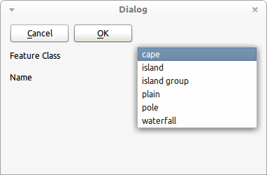
Note that here I have a QComboBox with the FeatureCla name, this will bind the combo box to the FeatureCla field in my dataset in QGIS.

Now set the custom form as the Edit UI for the layer

Set the Edit UI to your form

Tip: You can use relative paths if you store the form along side your project file

 Flick to the Fields tab and set up the Edit Widget type for each field that you have used on the custom feature form.

Set the Edit Widget that matches your control

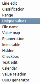
I have set the FeatueCla field to use Unique values widget, this tells QGIS to collect all the unique values from that column and add them to the QComboBox.  There are a range of different edit widgets you can set

Each will map to a different set of control types (Widgets) e.g. If you want to have a checkbox on your form you must select Checkbox in the Edit Widget list to get it to bind correctly.

Save the properties and head back to you map.  Use the Identify Tool to select a feature.

Values bound to form

And that is it. Pretty cool hey!

Final thoughts

This is one feature I really like in QGIS.  The ability to create custom forms for people to do data entry without the need to build a plugin is very cool.  Couple this the built-in GPS module for QGIS and you have yourself a nice simple field data collection program.

I have some ideas to make this feature even more powerful, but more on that later once I get some time to add it in.

Ok the title is a bit of a lie. QGIS did support MS SQL Server 2008 before by using OGR but this is a native provider so it’s a lot more integrated..

Good news everyone!

QGIS now has a native MS SQL 2008 provider. The provider can found using the new toolbar button (purple icon) or in the MS SQL node in the QBrowser tree. The provider also supports drag and drop import.

The work was sponsored by Digital Mapping Solutions (Australia) and completed by Tamas Szekeres

Any bugs can be assigned to “tamas” on hub.qgis.org.

A big thanks to both Digital Mapping Solutions and Tamas.

This addition will open QGIS up to a whole new set of users who have to use MS SQL but love QGIS.

Currently this is only in master but I will be in the 1.8 release when it comes out.

Note: At the moment you have to have a geometry_columns table in the database in order to connect, this table is the same format used by PostGIS and can be made by importing a layer using the ogr2ogr method. There will be a fix coming for this at some stage.

Did you know QGIS is also on all the major social networking sites?

No?

Well now you do :)

Google+
Facebook
Twitter

Search for QGIS on Twitter
Search for QGIS on Google+

Come join the discussions on your preferred platform. If you prefer not to say much, social networks are still a great way to keep up to date with all the cool stuff happening in QGIS land.

Anita Graser, of underdark.wordpress.com, and myself manage the Google+ and Facebook pages.

If you have something cool that you have done with QGIS and would like to pimp it to the world, free feel to contact me, or even just mention QGIS in the post, Mentioning QGIS will make it show up in the search on Twitter or Google+.  I keep a keen eye on all sites for anything cool that I can reshare on the main QGIS pages.

Gary Sherman has just published a new Python plugin for QGIS that I think people will find very handy, I know I will.  The plugin allows you to run Python scripts inside QGIS for tasks that don’t really require, or warrant, a whole plugin.

Go check out Gray’s post about the new plugin at http://spatialgalaxy.net/2012/01/29/script-runner-a-plugin-to-run-python-scripts-in-qgis/

The new plugin can be installed via the Plugin Installer using the “runner” or “script”.  The Plugin Installer is another one of my favorite plugins for QGIS, being able to push out a new plugin and know that everyone can get it is a good feeling :)

Following up on my last post, Running Scripts in the Python Console, I created a plugin to simplify running scripts:

The Script Runner plugin allows you to add your scripts to a list so they are readily available. You can then run them to automate QGIS tasks and have full access to the PyQGIS API. In addition, you can view information about the classes, methods, and functions in your module as well as browse the source:

In order for your script to work with ScriptRunner it has to implement a single function as an entry point. Here is some additional information from the Help tab of the plugin:

Requirements

In order for Script Runner to execute your script you must define a run_script function that accepts a single argument. This is the standard entry point used by Script Runner. A reference to the qgis.utils.iface object will be passed to your run_script function. You don’t have to use the iface object in your script but your run_script function must accept it as an argument.

Here is an example of a simple run_script function:

    def run_script(iface):
        ldr = Loader(iface)
        ldr.load_shapefiles('/vmap0_shapefiles')

In this example, the run_script creates an instance (ldr) of a class named Loader that is defined in the same source file. It then calls a method in the Loader class named load_shapefiles to do something useful—in this case, load all the shapefiles in a specified directory.

Alternatively, you could choose not to use classes and just do everything within the run_script function, including having it call functions in the same script or others you might import. The important thing is to be sure you have defined a run_script function. If not, Script Runner won’t load your script.

Working with Scripts

To run a script, you must add it to Script Runner using the Add Script tool on the toolbar. This will add it to a list in the left panel. This list of scripts is persisted between uses of QGIS. You can remove a script using the Remove Script tool. This just removes it from the list; it does nothing to the script file on disk.

Once you have a script loaded, you can click the Script Info tool to populate the Info and Source tabs in the panel on the right. The Info tab contains the docstring from your module and then a list of the classes, methods, and functions found in the script. Having a proper docstring at the head of your script will help you determine the puprose of script.

You can view the source of the script on the Source tab. This allows you to quickly confirm that you are using the right script and it does what you think it will.

Installing the Plugin

To install the plugin:

1. Open the Python plugin installer: Plugins->Fetch Python Plugins
2. Check to see if you have the new Official repository in your list of plugins by clicking on Repositories tab. The URL is http://plugins.qgis.org/plugins/plugins.xml.
3. If you have it, skip to step 5. If the new repository isn’t in the list, add it by clicking the Add button. Give it a name and insert the URL http://plugins.qgis.org/plugins/plugins.xml
4. Click on the Plugins tab
5. Enter scriptrunner in the Filter box
6. Select the ScriptRunner plugin and click Install

ScriptRunner adds an entry to the Plugins menu as well as a tool on the Plugins toolbar: . Click it and you are off and running.

The QGIS Python console is great for doing one-off tasks or experimenting with the API. Sometimes you might want to automate a task using a script, and do it without writing a full blown plugin. Currently QGIS does not have a way to load an arbitrary Python script and run it¹. Until it does, this post illustrates a way you can create a script and run it from the console.

There are a couple of requirements to run a script in the console:

1. The script must be in your PYTHONPATH
2. Just like a QGIS plugin, the script needs a reference to qgis.utils.iface

Setting up the Environment

By default, the Python path includes the .qgis/python directory. The location depends on your platform:

• Windows: in your home directory under .qgis\python. For example, C:\Documents and Settings\gsherman\.qgis\python
• Linux and OS X: $HOME/.qgis/python

To see what is in your PYTHONPATH you can do the following in QGIS Python console:

import sys
sys.path

While you could use the .qgis\python directory for your custom scripts, a better way is to create a directory specifically for that purpose and add that directory to the PYTHONPATH environment variable. On Windows you can do this using the Environment Variables page in your system properties:

On Linux or OS X, you can add it to your .bash_profile, .profile, or other login script in your home directory:

export PYTHONPATH=$PYTHONPATH:/home/gsherman/qgis_scripts

Writing the Script

With the environment set, we can create scripts to automate QGIS tasks and run them from the console. For this example, we will use a simple script to load all shapefiles in a specified directory. There are a couple of ways to do this:

1. Write a simple script with a function that accepts qgis.utils.iface as an argument, along with a path to the shapefiles
2. Create a Python class that uses an __init__ method to store a reference to the iface object and then add methods to do the work

We will use the latter approach because it is more flexible and allows us to initialize once and then call methods without having to pass the iface object each time.

The script looks like this:

#!/usr/bin/env Python
"""Load all shapefiles in a given directory.
  This script (loader.py) runs from the QGIS Python console.
  From the console, use:
    from loader import Loader
    ldr = Loader(qgis.utils.iface)
    ldr.load_shapefiles('/my/path/to/shapefile/directory')
 
  """
from glob import glob
from os import path
 
class Loader:
    def __init__(self, iface):
        """Initialize using the qgis.utils.iface 
        object passed from the console.
 
        """
        self.iface = iface
 
    def load_shapefiles(self, shp_path):
        """Load all shapefiles found in shp_path"""
        print "Loading shapes from %s" % path.join(shp_path, "*.shp")
        shps = glob(path.join(shp_path, "*.shp"))
        for shp in shps:
            (shpdir, shpfile) = path.split(shp)
            self.iface.addVectorLayer(shp, shpfile, 'ogr' )

Running the Script

To open the console use the Plugins->Python Console menu item.

The comment at the head of the script explains how to use it.

First we import the Loader class from the script file (named loader.py). This script resides in the qgis_scripts directory that is our PYTHONPATH.

from loader import Loader

We then create an instance of Loader, passing it the reference to the iface object:

ldr = Loader(qgis.utils.iface)

This creates the Loader object and calls the __init__ method to initialize things.

Once we have an instance of Loader we can load all the shapefiles in a directory by calling the load_shapefiles method, passing it the full path to the directory containing the shapefiles:

ldr.load_shapefiles('/home/gsherman/qgis_sample_data/vmap0_shapefiles')

The load_shapefiles method uses the path to get a list of all the shapefiles and then adds them to QGIS using addVectorLayer.

Here is the result, rendered in the random colors and order that the shapefiles were loaded:

Some Notes

• When testing a script in the console you may need to reload it as you make changes. This can be done using reload and the name of the module. In our example, reload(loader) does the trick.
• You can add more methods to your class to do additional tasks
• You can create a “driver” script that accepts the iface object and then initializes additional classes to do more complex tasks

1. I have plans on the drawing board to implement this feature.

The raster calculator allows you to perform mathematical operations on each cell in a raster. This can be useful for converting and manipulating your rasters. Operators include:

• Mathematical (+, -, *, /)
• Trigonometric (sin, cos, tan, asin, acos, atan)
• Comparison (<, >, =, <=, >=)
• Logical (AND, OR)

To perform operations on a raster or rasters, they must be loaded in QGIS. The raster calculator is accessed from the Raster menu and brings up the dialog:

Let’s look a few examples.

Simple Mathematical Calculation

Doing a simple calculation is easy. In this example we have a Digital Elevation Model (ancc6) loaded in QGIS. The DEM contains elevations for a 1:63,360 quadrangle in Alaska. The coordinate system is geographic and the elevation value in each cell is in meters. If we wanted to create a raster with elevation in feet, we can use these steps to create the expression:

1. Bring up the raster calculator
2. Double click on ancc6@1 in the raster bands list to add it to the expression
3. Double click the multiplication operator (*)
4. In the expression box, type in the conversion factor for meters to feet: 3.28

This gives us the following expression:

ancc6@1 * 3.28

To complete the process, we specify a name for the output raster and the format we want to use. When you click OK, the operation will be performed and the new raster created, giving us a GeoTIFF with cell values in feet. If you leave the Add result to project box checked the output raster will be added to QGIS once the calculations are done.

If you only want to operate on a portion of a raster, you can use the extent setting to limit the area included in the calculation.

Using a Mask

Sometimes you might want to mask out part of a raster. An example might be one where you have elevations ranging from below sea level to mountain tops. If you are only interested in elevations above sea level, you can use the raster calculator to create a mask and apply it to your raster all in one step.

The expression looks like this:

(my_raster@1 >= 0) * my_raster@1

The first part of the expression in parentheses effectively says: for every cell greater than or equal to zero, set its value to 1, otherwise set it to 0. This creates the mask on the fly.

In the second part of the expression, we multiply our raster (my_raster@1) by the mask values. This sets every cell with an elevation less than zero to zero. When you click OK, the calculator will create a new raster with the mask applied.

Simulating a Rise in Seal Level

Using the raster calculator and a mask we can visually simulate a rise in sea level. To do this we simply create the mask and overlay it on the DEM or perhaps a DRG (topographic) raster.

The expression to raise sea level by 100 meters is:

ancc6@1 > 100

The output raster contains cells with either a 0 (black) or 1 (while) value:

The black areas represent everything below an elevation of 100 meters, effectively illustrating a sea level rise. When we combine this with a suitable background we can demonstrate the results:

We added the DRG for the quadrangle and overlaid it with the mask layer. Setting the transparency to 70% allows the DRG to be seen, illustrating the effect of raising sea level.

The raster calculator is a powerful tool. Check it out and see how you might use it in your analysis and map making.

The rule based rendering in QGIS has just got a make over to improve in some of the old usability issues it used to have.  Most of the improvements are UI related. If you would like to try them out you will need to grab a copy of the latest dev build (qgis-dev in OSGeo4W)

Main improvements include:

• Nested rules.  If the parent rule evaluates to false none of the child rules are applied. This replaces the priority system in the old dialog.
• Disable symbol for rules. Rules with no symbol only act as a check for the child rules e.g nothing is rendered for the rule but child rules still are (unless also disabled).
• Drag and Drop rules (multi-selection is supported).  Rules can be dragged onto other rules in order to nest them and set up a rendering hierarchy.
• Inline editing of rule labels, expressions, scales
• Overall tweaks to the dialog

The new rule dialog

As you can see in the screenshot, the rules are now organized in a tree which clearly expresses which rules should be applied and when.

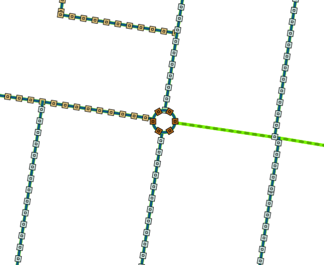
In the example above, all the rules under the Sealed rule will only be applied if that rule is true. The old system would have you managing all rules in one big list and dealing with priorities in order to get the rules to apply right, the new dialog is a major improvement.

And the results! As you can see below, QGIS will only render the colored squares if the Sealed rule is true otherwise it just shows a green line.

The rules applied

The work was sponsored by Ville de Morges, Switzerland and developed by Martin Dobias.  Thanks to both of them for these improvements.

More info:

• See Martin’s notes for a more detailed breakdown, and maybe some future stuff to come, of the improvements  http://lists.osgeo.org/pipermail/qgis-developer/2012-January/017909.html

Note: As this is a brand new feature there might be some bugs, or things that don’t quite work as expected. If you do find something don’t hesitate to file a bug report at hub.qgis.org so it can be fixed, or at least known about.

Good news!

Support for MS SQL Server 2008 in QGIS is coming soon.   A native QGIS provider for MS SQL Server is currently being worked on to make using, managing, and editing SQL Server data in QGIS just as easy as PostGIS.

The work is being sponsored by the Australian company Digital Mapping Solutions. So a very big thanks to them for this great feature!

There is no ETA on when it will be added to the main QGIS build, but the provider is currently in testing stage and hopefully will be in there soon.

So if you have been itching to try SQL Server data in QGIS, hang in there as a good solution is just around the corner.

P.S The other blog posts on this topic I used ogr, this method will still work fine after the native provider is added, however the native driver will add a nicer interface including integration into the QBrowser, better optimization for the QGIS code, and hopefully same feel as the PostGIS experience.

This week we look at the OpenLayers plugin for QGIS. This plugin allows you to add a number of image services to your map canvas:

• Google
• Physical
• Streets
• Hybrid
• Satellite
• OpenStreetMap
• Yahoo
• Street
• Hybrid
• Satellite
• Bing
• Road
• Aerial
• Aerial with labels

Installing the Plugin

The OpenLayers plugin is installed like all other Python plugins. From the the Plugins menu in QGIS, choose Fetch Python Plugins. This brings up the plugin installer. To find the plugin, enter openlayers in the Filter box, then select OpenLayers Plugin from the list. Once it’s highlighted, click the Install plugin button. This will download the plugin from the repository, install it, and load it into QGIS.

Using the Plugin

The OpenLayers Plugin uses your view extent to fetch the data from the service you choose. For this reason you should load at least one of your own layers first. Since each of the services are expecting a request in latitude/longitude your layer either has to be geographic or you must enable on the fly projection.

To add one of the services you have two choices; you can pick the service from the Plugins->OpenLayers plugin menu or you can use the OpenLayers Overview. The Overview opens a new panel that allows you to choose a service from a drop-down list. Click the Enable map checkbox to enable the drop-down list and preview the service you want to add. If you are happy with what you see, you can add it to the map by clicking the Add map button.

In the screenshot below we have enabled the Overview panel, added the world boundaries layer¹, zoomed to an area of interest, and added the Google terrain (physical) data:

You can add as many services as you want, previewing them using the OpenLayers Overview panel.

¹ You can get the world boundaries layer from the Geospatial Desktop sample data set.

This week we take a look at a how to plot a terrain profile using the Profile plugin. The plugin can be used with any raster format supported by QGIS. You can can display profiles from up to three rasters at once, allowing you to compare the results. To illustrate, we’ll create a simple profile using a DEM of a 1:63,360 quadrangle in Alaska.

Installing the Plugin

The Profile plugin is installed like all other Python plugins. From the the Plugins menu in QGIS, choose Fetch Python Plugins. This brings up the plugin installer. To find the plugin, enter profile in the Filter box, then select Profile from the list. Once it’s highlighted, click the Install plugin button. This will download the plugin from the repository, install it, and load it into QGIS.¹

Using the Plugin

Here we have loaded the DEM as well as a raster (DRG) of the topography for the same quadrangle and zoomed in a bit to an area of interest:

The yellow line has been added to indicate where we will take the profile. While the Profile plugin allows you to interactively select the profile line it doesn’t display the line on the map.

To create a profile, first make sure the raster you want to profile is selected in the layer list, then activate the plugin from the Plugins toolbar by clicking on it. The cursor becomes a cross that you use to create the profile line: click at the start point, move to the end and click again. Once you have created the profile line, the plugin pops up the result:

The profile is taken from the northeast towards the southwest, based on where we clicked first. You can change the exaggeration of the profile by using the slider on the left. The X axis shows the distance along the profile line in map units and the Y axis shows the cell values from the raster—in this case, elevation in meters.

You can save the result as a PDF or SVG using the buttons at the bottom of the dialog.

The Statistics tab displays some information for the raster layer and the profile line:

If we had additional rasters loaded, we could use the Setup tab to add them to the profile analysis. This would display the results using the colors specified for each layer and we could compare them on the Profile tab.

This is just one of several QGIS plugins that deal with profiles. You can check out the rest of them using the Python Plugin installer.

1 The Profile plugin requires the Python module for QWT5. If you don’t have this installed, a warning will be displayed during the installation process.

This week we highlight the Points to Paths plugin, a handy way to convert a series of points into line features. This plugin lets you “connect the dots” based on an common attribute and a sequence field. The attribute field determines which points should be grouped together into a line. The sequence field determines the order in which the points will connected. The output from this plugin is a shapefile.

Let’s take a look at some example data. Here we have some fictional wildlife tracking data for two moose. The tracking data is in shapefile format, but you can use any vector format supported by QGIS. The tracking data is symbolized by our two animals: Moose1 and Moose2:

The moose_tracks layer has an animal tracking id field (animal_tid) and a sequence field (id). This is all we need to convert the individual observations into a line feature that represents the animals path.

Installing the Plugin

The Points to Paths plugin is installed like all other Python plugins. From the the Plugins menu in QGIS, choose Fetch Python Plugins. This brings up the plugin installer. To find the plugin, enter points to in the Filter box, then select Points to Paths from the list. Once it’s highlighted, click the Install plugin button. This will download the plugin from the repository, install it, and load it into QGIS.

Using the Plugin

Let’s convert the tracking data to paths. To get started, choose Plugins->Points to Paths from the menu or click on the Points to Paths tool on the Plugin toolbar. This brings up the PointsToPaths dialog box where we specify the paramaters needed to create the paths. Below is the completed dialog for our moose tracks:

The first drop-down box contains a list of the vector layers loaded in QGIS—in our case we have just one: moose_tracks. For the group field drop-down we chose the field that contains the tracking identifier for each animal. This determines which points will be selected and grouped to form an individual line. The point order field drop-down specifies the field that contains the ordering for the observations. In this case, the id field is incremented with each observation and can be used to construct the paths. We don’t have a date/time field in this data, but your observations may be sequenced in this way. The Python date format field allows you to specify a format string so the plugin can determine how to sequence your points based on date/time.

The last thing we need to specify is the output shapefile. You can do this by typing in the full path to a new shapefile or by using the Browse button.

With these options set, clicking the OK button will create the new shapefile containing the paths created from our point observations. Once the shapefile is created, the plugin gives you the option to add the new shapefile directly to QGIS.

The Result

The result of our simple example are shown below:

We symbolized the individual tracks using the Categorized renderer on the Style tab of the vector properties dialog. You can see we now have a track for each animal. The attribute table created by the plugin contains the following fields:

• group – the name of the animal taken from the field we chose as the group field
• begin – the value of the first point order field used to create the path
• end – the value of the last point order field used to create the path

In our data, group contains the animal name, begin the value of the lowest id field for animal, and end contains the greatest id value. In a more typical data set, begin and end would contain the start and end date/time values for the observation. Labeling the observation points with our sequence field or date/time values would allow us to determine the direction of movement.

If you have point data that represent a movement of an object, this plugin is a great way to convert it into a path that can be used for visualization, analysis, or map composition.

QGIS has a lot of plugins, including over 180 that have been contributed by users. If you aren’t using plugins, you are missing out on a lot that QGIS has to offer. I’m starting what I hope to be a regular feature: Plugin of the Week. This week we’ll take a look at Time Manager.

Time Manager lets you browse spatial data that has a temporal component. Essentially this includes anything that changes location through time. Examples include:

• Wildlife tracking
• Vehicles
• Storm centers
• QGIS users

Data Preparation

Expanding on our last post about QGIS Users Around the World, we’ll use Time Manager to watch access to the QGIS Python plugin repository through time. If you refer to the previous post, you’ll see that all the IP addresses contacting the repository were extracted from the web server log and geocoded to get the approximate geographic coordinates. To use Time Manager all we need is the time for each access to the repository.

A important part (for our purpose) of the web server log entry looks like this:

66.58.228.196 - - [23/Oct/2011:21:17:54 +0000] "GET /repo/contributed HTTP/1.1" 200 256

Time Manager supports date/time in the following formats:

• YYYY-MM-DD HH:MM:SS
• YYYY-MM-DD HH:MM
• YYYY-MM-DD

As you can see, this doesn’t work with the format in the web server log.

The geocoding process created a file containing IP address, country, city (where available), latitude and longitude. This file is used to create a Python dictionary to look up locations by IP address. Using this file and a bit of Python, the web server log entries were converted into a CSV file containing:

ip,date_time,country,latitude,longitude
66.58.228.196,2011-10-23 21:13:53,United States,61.2149,-149.258
66.58.228.196,2011-10-23 21:14:22,United States,61.2149,-149.258
66.58.228.196,2011-10-23 21:17:54,United States,61.2149,-149.258
66.58.228.196,2011-10-23 21:18:04,United States,61.2149,-149.258
...


The CSV file was first converted to a shapefile using the QGIS Delimited Text plugin. Performance with Time Manager was somewhat slow using a shapefile containing 134,171 locations. The shapefile was imported into a SpatiaLite database (you can do this using ogr2ogr or the SpatiaLite GUI).

Using Time Manager

To display the progression of access to the repository (and thus users of QGIS), we first have to have the Time Manager plugin installed.^[1] Once installed, we enable it using the Plugin Manger.

As you can see from the screenshot above, Time Manager installs a new panel in QGIS that sits below the map canvas. You can set a number of options by clicking Settings; the most important being the layer to use in the visualization. For the QGIS users, we use the time_manager_req layer that was created from the web server logs. With the location and date/time data in the proper format, you can click the “Play” button to start the display. For each time interval, the plugin selects the appropriate entries and displays a frame for the duration specified in the settings.

You can use the time slider to move around or move the time interval forward or backward using the buttons on each end of the slider.

A really nice feature is the ability to export to video. At present this saves a PNG file and world file for each time interval. You can then use another software package to combine these to create a video animation of the time sequence. Once solution is to use mencoder^[1]:

mencoder "mf://*.PNG" -mf fps=10 -o output.avi -ovc lavc -lavcopts vcodec=mpeg4

Putting all this together gives us the following visualization of QGIS user activity from October 23 through December 19, 2011:

QGIS User Activity

You can see the “wave” of activity progress from east to west as the daylight hours come and go.

Summary

If you have spatial data with a date or time component, the Time Manager plugin provides a convenient way to visualize the temporal relationships.

[1]http://www.geofrogger.net/trac/wiki

One of the difficult things to track in the open source world is the number of people who actually use your software. In the proprietary commercial world you have licenses, invoices, and so forth. In the case of QGIS, we can track the total number of downloads from qgis.org, but this doesn’t represent the total installed base. It is impossible to accurately determine the actual number of people using QGIS, but we can get an approximation of the number and where they are in the world.

The analysis was done using the log files from the QGIS contributed repository:

• The IP address of each entry that retrieved the plugin list from the server represents one or more users—these IPs were collected into a unique list
• Using a Python script, each IP address in the log was geocoded to get the approximate latitude and longitude of the user
• The IP address, country, latitude, and longitude were written to a CSV file
• The CSV file was converted to a Spatialite layer to create the map of users

The map represents 35,603 unique IP addresses of users that accessed the repository between October 23, 2011 and December 17, 2011.

The geocoding process varies in precision—some IPs are located to the city level while others only return a general location for the country.

Some assumptions and observations:

• Most (maybe all) users make use of Python plugins and therefore access the contributed repository at some point
• Country-level points (blue) on the map represent more than one user
• Some points represent organizations that use a single IP for all users accessing the Internet. These points will represent more than one user
• Some users may access the repository from more than one IP address

So how many people use QGIS? At the very minimum, 35,000. We know that the downloads of just the Windows version exceeded 100,000. Given that there are 7,183 IP addresses that are generalized to a country location, we can safely assume that the number of actual users is much higher than that.

Considering the number of points that represent an organization and those that represent a country location, I think we can safely assume that the number of QGIS users easily exceeds 100,000 worldwide.

This post is for those of you that build QGIS on a regular basis and want to keep up with everything going on in the current release branches (1.7.2 and 1.8) as well as the master branch that will eventually become version 2.0.

While you can do all your work in one clone, this method has a couple of advantages, at the expense of a bit of disk space:

1. Quicker compiles compared to branch switching, especially if you are using ccache
2. Less likelihood of making a merge mess when switching branches

The basic steps are:

1. Login to github and clone the QGIS repository (https://github.com/qgis/Quantum-GIS)
2. Create a working copy of your github clone on your machine
3. Add a reference to the upstream repository
4. Fetch and merge (if required) from the upstream repository
5. Create a new clone for the branch by cloning the working copy created in step 2
6. Change to the branch clone directory
7. Add the upstream remote
8. Fetch from upstream
9. Create the tracking branch
10. Checkout the branch

It’s simpler than it sounds—the following steps should work on any platform and assume you have already created your own clone of the QGIS repository on github.

First make a directory for development, change to it, and fetch a copy of your clone of QGIS from github (this will take a while):

gsherman@dork:~$ mkdir qgis_dev
gsherman@dork:~$ cd qgis_dev
gsherman@dork:~/qgis_dev$ git clone [email protected]:g-sherman/Quantum-GIS.git
Cloning into Quantum-GIS...
remote: Counting objects: 183812, done.
remote: Compressing objects: 100% (42255/42255), done.
remote: Total 183812 (delta 140627), reused 183281 (delta 140221)
Receiving objects: 100% (183812/183812), 240.80 MiB | 1.19 MiB/s, done.
Resolving deltas: 100% (140627/140627), done.


Now change to your new clone directory and add the upstream repository (the QGIS repo on github):

gsherman@dork:~/qgis_dev$ cd Quantum-GIS/
gsherman@dork:~/qgis_dev/Quantum-GIS$ git remote add upstream [email protected]:qgis/Quantum-GIS.git

We can then list our config to see that the remote was added:

gsherman@dork:~/qgis_dev/Quantum-GIS$ git config --list
core.repositoryformatversion=0
core.filemode=true
core.bare=false
core.logallrefupdates=true
remote.origin.fetch=+refs/heads/*:refs/remotes/origin/*
[email protected]:g-sherman/Quantum-GIS.git
branch.master.remote=origin
branch.master.merge=refs/heads/master
[email protected]:qgis/Quantum-GIS.git
remote.upstream.fetch=+refs/heads/*:refs/remotes/upstream/*


Then we do a fetch from the QGIS repo to make sure things are up to date:

gsherman@dork:~/qgis_dev/Quantum-GIS$ git fetch upstream


If your clone of the QGIS repository on github is not brand new, you should do a merge before proceeding:

gsherman@dork:~/qgis_dev/Quantum-GIS$ git merge upstream/master


Now we can create a new clone for the 1.7.2 branch using our local master:

gsherman@dork:~/qgis_dev/Quantum-GIS$ cd ..
gsherman@dork:~/qgis_dev$ git clone ./Quantum-GIS Quantum-GIS-1_7_2
Cloning into Quantum-GIS-1_7_2...
done.


Now we need to add the remote for the main QGIS repository:

gsherman@dork:~/qgis_dev$ cd Quantum-GIS-1_7_2/
gsherman@dork:~/qgis_dev/Quantum-GIS-1_7_2$ git remote add upstream [email protected]:qgis/Quantum-GIS.git


The next step is to fetch from upstream to make sure we have references to the branches:

gsherman@dork:~/qgis_dev/Quantum-GIS-1_7_2$ git fetch upstream
* [new branch] dev-threading -> upstream/dev-threading
* [new branch] master -> upstream/master
* [new branch] release-0_0_11 -> upstream/release-0_0_11
* [new branch] release-0_0_12 -> upstream/release-0_0_12
...
* [new branch] release-1_7_1 -> upstream/release-1_7_1
* [new branch] release-1_7_2 -> upstream/release-1_7_2
* [new branch] release-1_8 -> upstream/release-1_8

Now we create the branch to track the release of interest—in this case 1.7.2:

gsherman@dork:~/qgis_dev/Quantum-GIS-1_7_2$ git branch --track release-1_7_2 upstream/release-1_7_2
Branch release-1_7_2 set up to track remote branch release-1_7_2 from upstream.

The last step is to check out the branch which should go pretty quick:

gsherman@dork:~/qgis_dev/Quantum-GIS-1_7_2$ git checkout release-1_7_2
Checking out files: 100% (1809/1809), done.
Switched to branch 'release-1_7_2'

You are now ready to build the 1.7.2 release branch. Repeat the process for any other branches you want to track.

The Plugin Builder allows you to quickly create a skeleton Python plugin by generating all that boring boilerplate that every plugin requires.

Here is a short video showing how to create, compile, and install a new plugin.

For more information, see QGIS Workshop Documentation and the PyQGIS Cookbook.

QGIS finally has expression based labels! (Although you must be running latest dev build)

What does that mean? Well QGIS used to be only able to label with a field from the layer, very limiting if you need to make a nice looking label string. Now you can use expressions (eg ‘Up ‘ || US_Invert || ‘some more text’ ) to label the feature, just like this.

Example of expression based labels

This is something that I missed a lot when moving from MapInfo to QGIS.  After opening a ticket on the QGIS bug list and nothing happening with it for a couple of months (not that I expected anything to, everyone is busy enough as is.  I don’t expect the devs to just jump at all my requests) so I decided I should at least attempt adding it myself.  The joys of open source!

Turns out adding the expression labeling was the easy part, however there was no good generic expression string builder that I could use to build the expression string.  QGIS already had the expression builder for the query window and the field calculator, however the code was very tied down to only work for those implementations, plus they didn’t scale with the increasing function list.  I’m not going to go and make yet another dialog just for the labeling.  Uniformity is the key to good user experience.

After searching around to see what other GIS systems did to get some inspiration it seemed that every example that I came across was, in my opinion, poor.    Although there was one ArcGIS idea ticket that gave me a few ideas http://ideas.arcgis.com/ideaView?id=087300000008IbHAAU

So with that I started working on a generic expression builder that could be used to build an expression string anywhere, replacing the query window and field calculator in due time. One ring widget to rule them all, one ring widget to bind the, etc.

The result

Generic expression builder

Key features of the new expression builder:

• Live validation of expression
• Real time searching
• Live output preview
• Help on selected item.
• Easier to add new functions without changing the UI.  Function list is read right from the expression parser.  No more hidden functions.
• Reusable widget

If the expression hits an error while you type you will be shown an “Expression is invalid” warning (yes I know it’s wrong in the screen shot). Clicking (more info) or hovering over the expression area will show you the error.

Expression has error

Searching can done by using the search box at the top. The function list will reduce to show only functions or fields containing that string (Note: it is case sensitive at the current time) .

Searching for a function or field name.

Still to do

As with all programming it is never bug free so I expect, now that it is open to wider testing, that there might be a few that need to be addressed .   There is also very limited function help written for the functions, although if anyone is willing to have a go at it I’m more than happy.

If you do find any bugs will the widget/dialog you can open a ticket at http://hub.qgis.org/projects/quantum-gis/issues , assign it to me and I’ll see what I can do.

In the works

• Simple Syntax highlighting
• Recent expression used list
• Saved expressions
• Auto bracketing (maybe)
• UI tweaking

I would like to thank Martin from the QGIS team for reviewing my code all though the project and helping me improve the code and idea.  Also thanks to all the other people who gave ideas for the widget/dialog.

Enjoy!

I tell you. It always amazes me how much cool stuff you can do with great open source GIS software these days. GDAL is one of those great open source projects that I have just found a great use for (apart from just opening every raster type under the sun in QGIS).

GDAL has the ability to generate contours from a DEM, something that I have always wanted to try for my town but have never been able due to lack of a good DEMs.

Recently we purchased a set of DEMs that cover a large area as part of a study. Each DEM uses a grid size of 1mx1m. Prefect for generating contours.

Using the GdalTools QGIS plugin.

First make sure that you have the latest version of the GdalTools plugin installed (GdalTools should be installed by default with QGIS. If it’s not, search “Gdal” in the plugin installer). Enable the plugin once it’s installed.

Load the DEM into QGIS using the Load Raster icon.

DEM loaded in QGIS

Now head up to the menu Raster->Extraction->Contour

Raster menu in QGIS

Select the settings that you need. For this DEM I am going to generate 250mm contours.

Contour dialog.

Take note of the text area at the bottom of the dialog as that is the exact command sent to GDAL in order to generate the contours. If you take a copy of that you can run it on the command line for batch processing later.

Hit ok.

250mm contours from the DEM

BAM! :)

Using the command line/shell.

Using QGIS for a one off DEM is fine and dandy but what if you have 3000 DEMs that you need to process. To hell with doing that by hand!

Remember the contour tool in QGIS told us the exact command line args to use, so creating a shell script for automating the process is pretty easy.

for f in *.asc
do
  echo "Processing $f"
 gdal_contour -a ELEV -i 0.25 $f $f-250mm.shp
done

The above code will loop though the current directory and process all the DEMs generating 250mm contours for each one. It saves each new contour file as {filename}-250mm.shp. You will need to change *.asc to whatever format your DEM is in.

Copy the above code into a file somewhere and call it generate_contours.sh. This can then be called from the command line using

sh generate_contours.sh

Running sh on Windows

If you’re a windows user you will need to run OsGeo4W Shell in order to use sh.

Loading OsGeo4w shell.

Once the shell is loaded you can just call:

sh generate_contours.sh

Output from running generate_contours.sh

Final remarks

I ran the above sh script on a folder with about 2500 DEMs and it took around 4 hours to complete the whole folder. Of course performance will vary but it seems pretty quick considering.

Once again the possibly to use open source GIS tools to get my work done is amazing.  No expensive software here.

So far I’m not aware of any line smoothing/generalizing abilities using GDAL/OGR.  Although you can import the contours into GRASS and use that: http://grass.osgeo.org/wiki/V.generalize_tutorial

You can also generate the contours using GDAL via Python but that is a topic for another day.

I added a simple feature that allows you to search the IRC logs from #qgis back to May 10, 2006.

The search is case sensitive and will return a list of all matches. Not too smart but it will get you close to what you want.

See the link at http://irclogs.geoapt.com/qgis