Today’s post continues where “Why you should be using PostGIS trajectories” leaves off. It’s the result of a collaboration with Eva Westermeier. I had the pleasure to supervise her internship at AIT last year and also co-supervised her Master’s thesis [0] on the topic of enriching trajectories with information about their geographic context.

Context-aware analysis of movement data is crucial for different domains and applications, from transport to ecology. While there is a wealth of data, efficient and user-friendly contextual trajectory analysis is still hampered by a lack of appropriate conceptual approaches and practical methods. (Westermeier, 2018)

Part of the work was focused on evaluating different approaches to adding context information from vector datasets to trajectories in PostGIS. For example, adding land cover context to animal movement data or adding information on anchoring and harbor areas to vessel movement data.

Classic point-based model vs. line-based model

The obvious approach is to intersect the trajectory points with context data. This is the classic point data model of contextual trajectories. It’s straightforward to add context information in the point-based model but it also generates large numbers of repeating annotations. In contrast, the line data model using, for example, PostGIS trajectories (LinestringM) is more compact since trajectories can be split into segments at context borders. This creates one annotation per segment and the individual segments are convenient to analyze (as described in part #12).

Spatio-temporal interpolation as provided by the line data model offers additional advantages for the analysis of annotated segments. Contextual segments start and end at the intersection of the trajectory linestring with context polygon borders. This means that there are no gaps like in the point-based model. Consequently, while the point-based model systematically underestimates segment length and duration, the line-based approach offers more meaningful segment length and duration measurements.

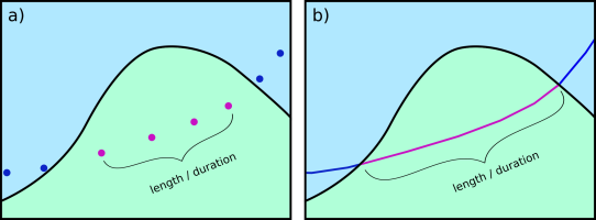
Schematic illustration of a subset of an annotated trajectory in two context classes, a) systematic underestimation of length or duration in the point data model, b) full length or duration between context polygon borders in the line data model (source: Westermeier (2018))

Another issue of the point data model is that brief context changes may be missed or represented by just one point location. This makes it impossible to compute the length or duration of the respective context segment. (Of course, depending on the application, it can be desirable to ignore brief context changes and make the annotation process robust towards irrelevant changes.)

Schematic illustration of context annotation for brief context changes, a) and b)
two variants for the point data model, c) gapless annotation in the line data model (source: Westermeier (2018) based on Buchin et al. (2014))

Beyond annotations, context can also be considered directly in an analysis, for example, when computing distances between trajectories and contextual point objects. In this case, the point-based approach systematically overestimates the distances.

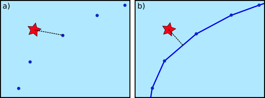
Schematic illustration of distance measurement from a trajectory to an external
object, a) point data model, b) line data model (source: Westermeier (2018))

The above examples show that there are some good reasons to dump the classic point-based model. However, the line-based model is not without its own issues.

Issues

Computing the context annotations for trajectory segments is tricky. The main issue is that ST_Intersection drops the M values. This effectively destroys our trajectories! There are ways to deal with this issue – and the corresponding SQL queries are published in the thesis (p. 38-40) – but it’s a real bummer. Basically, ST_Intersection only provides geometric output. Therefore, we need to reconstruct the temporal information in order to create usable trajectory segments.

Finally, while the line-based model is well suited to add context from other vector data, it is less useful for context data from continuous rasters but that was beyond the scope of this work.

Conclusion

After the promising results of my initial investigations into PostGIS trajectories, I was optimistic that context annotations would be a straightforward add-on. The line-based approach has multiple advantages when it comes to analyzing contextual segments. Unfortunately, generating these contextual segments is much less convenient and also slower than I had hoped. Originally, I had planned to turn this work into a plugin for the Processing toolbox but the results of this work motivated me to look into other solutions. You’ve already seen some of the outcomes in part #20 “Trajectools v1 released!”.

References

[0] Westermeier, E.M. (2018). Contextual Trajectory Modeling and Analysis. Master Thesis, Interfaculty Department of Geoinformatics, University of Salzburg.

This post is part of a series. Read more about movement data in GIS.

PyQGIS scripts are great to automate spatial processing workflows. It’s easy to run these scripts inside QGIS but it can be even more convenient to run PyQGIS scripts without even having to launch QGIS. To create a so-called “stand-alone” PyQGIS script, there are a few things that need to be taken care of. The following steps show how to set up PyCharm for stand-alone PyQGIS development on Windows10 with OSGeo4W.

An essential first step is to ensure that all environment variables are set correctly. The most reliable approach is to go to C:\OSGeo4W64\bin (or wherever OSGeo4W is installed on your machine), make a copy of qgis-dev-g7.bat (or any other QGIS version that you have installed) and rename it to pycharm.bat:

Instead of launching QGIS, we want that pycharm.bat launches PyCharm. Therefore, we edit the final line in the .bat file to start pycharm64.exe:

In PyCharm itself, the main task to finish our setup is configuring the project interpreter:

First, we add a new “system interpreter” for Python 3.7 using the corresponding OSGeo4W Python installation.

To finish the interpreter config, we need to add two additional paths pointing to QGIS\python and QGIS\python\plugins:

That’s it! Now we can start developing our stand-alone PyQGIS script.

The following example shows the necessary steps, particularly:

1. Initializing QGIS
2. Initializing Processing
3. Running a Processing algorithm

import sys

from qgis.core import QgsApplication, QgsProcessingFeedback
from qgis.analysis import QgsNativeAlgorithms

QgsApplication.setPrefixPath(r'C:\OSGeo4W64\apps\qgis-dev', True)
qgs = QgsApplication([], False)
qgs.initQgis()

# Add the path to processing so we can import it next
sys.path.append(r'C:\OSGeo4W64\apps\qgis-dev\python\plugins')
# Imports usually should be at the top of a script but this unconventional 
# order is necessary here because QGIS has to be initialized first
import processing
from processing.core.Processing import Processing

Processing.initialize()
QgsApplication.processingRegistry().addProvider(QgsNativeAlgorithms())
feedback = QgsProcessingFeedback()

rivers = r'D:\Documents\Geodata\NaturalEarthData\Natural_Earth_quick_start\10m_physical\ne_10m_rivers_lake_centerlines.shp'
output = r'D:\Documents\Geodata\temp\danube3.shp'
expression = "name LIKE '%Danube%'"

danube = processing.run(
    'native:extractbyexpression',
    {'INPUT': rivers, 'EXPRESSION': expression, 'OUTPUT': output},
    feedback=feedback
    )['OUTPUT']

print(danube)

When QGIS 3.0 was release, I published a Processing script template for QGIS3. While the script template is nicely pythonic, it’s also pretty long and daunting for non-programmers. This fact didn’t go unnoticed and Nathan Woodrow in particular started to work on a QGIS enhancement proposal to improve the situation and make writing Processing scripts easier, while – at the same time – keeping in line with common Python styles.

While the previous template had 57 lines of code, the new template only has 26 lines – 50% less code, same functionality! (Actually, this template provides more functionality since it also tracks progress and ensures that the algorithm can be cancelled.)

from qgis.processing import alg
from qgis.core import QgsFeature, QgsFeatureSink

@alg(name="ex_new", label=alg.tr("Example script (new style)"), group="examplescripts", group_label=alg.tr("Example Scripts"))
@alg.input(type=alg.SOURCE, name="INPUT", label="Input layer")
@alg.input(type=alg.SINK, name="OUTPUT", label="Output layer")
def testalg(instance, parameters, context, feedback, inputs):
    """
    Description goes here. (Don't delete this! Removing this comment will cause errors.)
    """
    source = instance.parameterAsSource(parameters, "INPUT", context)

    (sink, dest_id) = instance.parameterAsSink(
        parameters, "OUTPUT", context,
        source.fields(), source.wkbType(), source.sourceCrs())

    total = 100.0 / source.featureCount() if source.featureCount() else 0
    features = source.getFeatures()
    for current, feature in enumerate(features):
        if feedback.isCanceled():
            break
        out_feature = QgsFeature(feature)
        sink.addFeature(out_feature, QgsFeatureSink.FastInsert)
        feedback.setProgress(int(current * total))

    return {"OUTPUT": dest_id}

The key improvement are the new decorators that turn an ordinary function (such as testalg in the template) into a Processing algorithm. Decorators start with @ and are written above a function definition. The @alg decorator declares that the following function is a Processing algorithm, defines its name and assigns it to an algorithm group. The @alg.input decorator creates an input parameter for the algorithm. Similarly, there is a @alg.output decorator for output parameters.

For a longer example script, check out the original QGIS enhancement proposal thread!

For now, this new way of writing Processing scripts is only supported by QGIS 3.6 but there are plans to back-port this improvement to 3.4 once it is more mature. So give it a try and report back!

In previous posts, I already wrote about Trajectools and some of the functionality it provides to QGIS Processing including:

• Creating trajectories from points
• Clipping trajectories by extent
• Splitting trajectories by date

There are also tools to compute heading and speed which I only talked about on Twitter.

Trajectools is now available from the QGIS plugin repository.

The plugin includes sample data from MarineCadastre downloads and the Geolife project.

Under the hood, Trajectools depends on GeoPandas!

If you are on Windows, here’s how to install GeoPandas for OSGeo4W:

1. OSGeo4W installer: install python3-pip
2. Environment variables: add GDAL_VERSION = 2.3.2 (or whichever version your OSGeo4W installation currently includes)
3. OSGeo4W shell: call C:\OSGeo4W64\bin\py3_env.bat
4. OSGeo4W shell: pip3 install geopandas (this will error at fiona)
5. From https://www.lfd.uci.edu/~gohlke/pythonlibs/#fiona: download Fiona-1.7.13-cp37-cp37m-win_amd64.whl
6. OSGeo4W shell: pip3 install path-to-download\Fiona-1.7.13-cp37-cp37m-win_amd64.whl
7. OSGeo4W shell: pip3 install geopandas
8. (optionally) From https://www.lfd.uci.edu/~gohlke/pythonlibs/#rtree: download Rtree-0.8.3-cp37-cp37m-win_amd64.whl and pip3 install it

If you want to use this functionality outside of QGIS, head over to my movingpandas project!

Yesterday, I learned about a cool use case in data-driven agriculture that requires dealing with delayed measurements. As Bert mentions, for example, potatoes end up in the machines and are counted a few seconds after they’re actually taken out of the ground:

Therefore, in order to accurately map yield, we need to take this temporal offset into account.

We need to make sure that time and location stay untouched, but need to shift the potato count value. To support this use case, I’ve implemented apply_offset_seconds() for trajectories in movingpandas:

    def apply_offset_seconds(self, column, offset):
        self.df[column] = self.df[column].shift(offset, freq='1s')

The following test illustrates its use: you can see how the value column is shifted by 120 second. Geometry and time remain unchanged but the value column is shifted accordingly. In this test, we look at the row with index 2 which we access using iloc[2]:

    def test_offset_seconds(self):
        df = pd.DataFrame([
            {'geometry': Point(0, 0), 't': datetime(2018, 1, 1, 12, 0, 0), 'value': 1},
            {'geometry': Point(-6, 10), 't': datetime(2018, 1, 1, 12, 1, 0), 'value': 2},
            {'geometry': Point(6, 6), 't': datetime(2018, 1, 1, 12, 2, 0), 'value': 3},
            {'geometry': Point(6, 12), 't': datetime(2018, 1, 1, 12, 3, 0), 'value':4},
            {'geometry': Point(6, 18), 't': datetime(2018, 1, 1, 12, 4, 0), 'value':5}
        ]).set_index('t')
        geo_df = GeoDataFrame(df, crs={'init': '31256'})
        traj = Trajectory(1, geo_df)
        traj.apply_offset_seconds('value', -120)
        self.assertEqual(traj.df.iloc[2].value, 5)
        self.assertEqual(traj.df.iloc[2].geometry, Point(6, 6))

Many current movement data sources provide more or less continuous streams of object locations. For example, the AIS system provides continuous locations of vessels (mostly ships). This continuous stream of locations – let’s call it track – starts when we first record the vessel and ends with the last record. This start and end does not necessarily coincide with the start or end of a vessel voyage from one port to another. The stream start and end do not have any particular meaning. Instead, if we want to see what’s going on, we need to split the track into meaningful segments. One such segmentation – albeit a simple one – is to split tracks by day. This segmentation assumes that day/night changes affect the movement of our observed object. For many types of objects – those who mostly stay still during the night – this will work reasonably well.

For example, the following screenshot shows raw data of one particular vessel in the Boston region. By default, QGIS provides a Points to Path to convert points to lines. This tool takes one “group by” and one “order by” field. Therefore, if we want one trajectory per ship per day, we’d first have to create a new field that combines ship ID and day so that we can use this combination as a “group by” field. Additionally, the resulting lines loose all temporal information.

To simplify this workflow, Trajectools now provides a new algorithm that creates day trajectories and outputs LinestringM features. Using the Day trajectories from point layer tool, we can immediately see that our vessel of interest has been active for three consecutive days: entering our observation area on Nov 5th, moving to Boston where it stayed over night, then moving south to Weymouth on the next day, and leaving on the 7th.

Since the resulting trajectories are LinestringM features with time information stored in the M value, we can also visualize the speed of movement (as discussed in part #2 of this series):

Pandas is great for data munging and with the help of GeoPandas, these capabilities expand into the spatial realm.

With just two lines, it’s quick and easy to transform a plain headerless CSV file into a GeoDataFrame. (If your CSV is nice and already contains a header, you can skip the header=None and names=FILE_HEADER parameters.)

usecols=USE_COLS is also optional and allows us to specify that we only want to use a subset of the columns available in the CSV.

After the obligatory imports and setting of variables, all we need to do is read the CSV into a regular DataFrame and then construct a GeoDataFrame.

import pandas as pd
from geopandas import GeoDataFrame
from shapely.geometry import Point

FILE_NAME = "/temp/your.csv"
FILE_HEADER = ['a', 'b', 'c', 'd', 'e', 'x', 'y']
USE_COLS = ['a', 'x', 'y']

df = pd.read_csv(
    FILE_NAME, delimiter=";", header=None,
    names=FILE_HEADER, usecols=USE_COLS)
gdf = GeoDataFrame(
    df.drop(['x', 'y'], axis=1),
    crs={'init': 'epsg:4326'},
    geometry=[Point(xy) for xy in zip(df.x, df.y)])

It’s also possible to create the point objects using a lambda function as shown by weiji14 on GIS.SE.

If you’ve been following my posts, you’ll no doubt have seen quite a few flow maps on this blog. This tutorial brings together many different elements to show you exactly how to create a flow map from scratch. It’s the result of a collaboration with Hans-Jörg Stark from Switzerland who collected the data.

The flow data

The data presented in this post stems from a survey conducted among public transport users, especially commuters (available online at: https://de.surveymonkey.com/r/57D33V6). Among other questions, the questionnair asks where the commuters start their journey and where they are heading.

The answers had to be cleaned up to correct for different spellings, spelling errors, and multiple locations in one field. This cleaning and the following geocoding step were implemented in Python. Afterwards, the flow information was aggregated to count the number of nominations of each connection between different places. Finally, these connections (edges that contain start id, destination id and number of nominations) were stored in a text file. In addition, the locations were stored in a second text file containing id, location name, and co-ordinates.

Why was this data collected?

Besides travel demand, Hans-Jörg’s survey also asks participants about their coffee consumption during train rides. Here’s how he tells the story behind the data:

As a nearly daily commuter I like to enjoy a hot coffee on my train rides. But what has bugged me for a long time is the fact the coffee or hot beverages in general are almost always served in a non-reusable, “one-use-only-and-then-throw-away” cup. So I ended up buying one of these mostly ugly and space-consuming reusable cups. Neither system seem to satisfy me as customer: the paper-cup produces a lot of waste, though it is convenient because I carry it only when I need it. With the re-usable cup I carry it all day even though most of the time it is empty and it is clumsy and consumes the limited space in bag.

So I have been looking for a system that gets rid of the disadvantages or rather provides the advantages of both approaches and I came up with the following idea: Installing a system that provides a re-usable cup that I only have with me when I need it.

In order to evaluate the potential for such a system – which would not only imply a material change of the cups in terms of hardware but also introduce some software solution with the convenience of getting back the necessary deposit that I pay as a customer and some software-solution in the back-end that handles all the cleaning, distribution to the different coffee-shops and managing a balanced stocking in the stations – I conducted a survey

The next step was the geographic visualization of the flow data and this is where QGIS comes into play.

The flow map

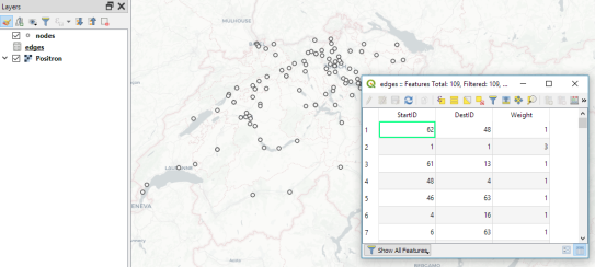
Survey data like the one described above is a common input for flow maps. There’s usually a point layer (here: “nodes”) that provides geographic information and a non-spatial layer (here: “edges”) that contains the information about the strength or weight of a flow between two specific nodes:

The first step therefore is to create the flow line features from the nodes and edges layers. To achieve our goal, we need to join both layers. Sounds like a job for SQL!

More specifically, this is a job for Virtual Layers: Layer | Add Layer | Add/Edit Virtual Layer

SELECT StartID, DestID, Weight, 
       make_line(a.geometry, b.geometry)
FROM edges
JOIN nodes a ON edges.StartID = a.ID
JOIN nodes b ON edges.DestID = b.ID
WHERE a.ID != b.ID 

This SQL query joins the geographic information from the nodes table to the flow weights in the edges table based on the node IDs. In the last line, there is a check that start and end node ID should be different in order to avoid zero-length lines.

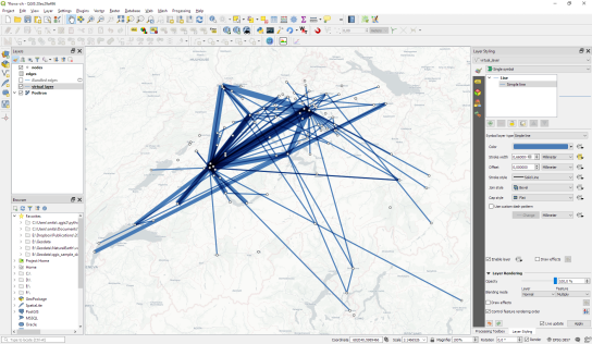
By styling the resulting flow lines using data-driven line width and adding in some feature blending, it’s possible to create some half decent maps:

However, we can definitely do better. Let’s throw in some curved arrows!

The arrow symbol layer type automatically creates curved arrows if the underlying line feature has three nodes that are not aligned on a straight line.

Therefore, to turn our straight lines into curved arrows, we need to add a third point to the line feature and it has to have an offset. This can be achieved using a geometry generator and the offset_curve() function:

make_line(
   start_point($geometry),
   centroid(
      offset_curve(
         $geometry, 
         length($geometry)/-5.0
      )
   ),
   end_point($geometry)
)

Additionally, to achieve the effect described in New style: flow map arrows, we extend the geometry generator to crop the lines at the beginning and end:

difference(
   difference(
      make_line(
         start_point($geometry),
         centroid(
            offset_curve(
               $geometry, 
               length($geometry)/-5.0
            )
         ),
	 end_point($geometry)
      ),
      buffer(start_point($geometry), 0.01)
   ),
   buffer(end_point( $geometry), 0.01)
)

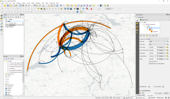
By applying data-driven arrow and arrow head sizes, we can transform the plain flow map above into a much more appealing map:

The two different arrow colors are another way to emphasize flow direction. In this case, orange arrows mark flows to the west, while blue flows point east.

CASE WHEN
 x(start_point($geometry)) - x(end_point($geometry)) < 0
THEN
 '#1f78b4'
ELSE
 '#ff7f00'
END

Conclusion

As you can see, virtual layers and geometry generators are a powerful combination. If you encounter performance problems with the virtual layer, it’s always possible to make it permanent by exporting it to a file. This will speed up any further visualization or analysis steps.

MovingPandas is my attempt to provide a pure Python solution for trajectory data handling in GIS. MovingPandas provides trajectory classes and functions built on top of GeoPandas. 

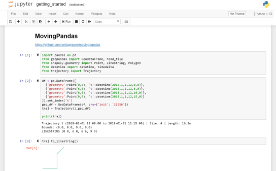
To lower the entry barrier to getting started with MovingPandas, there’s now an interactive iPython notebook hosted on MyBinder. This notebook provides all the necessary imports and demonstrates how to create a Trajectory object.

Launch MyBinder for MovingPandas to get started!

This post looks into the current AI hype and how it relates to geoinformatics in general and movement data analysis in GIS in particular. This is not an exhaustive review but aims to highlight some of the development within these fields. There are a lot of references in this post, including some to previous work of mine, so you can dive deeper into this topic on your own.

I’m looking forward to reading your take on this topic in the comments!

Introduction to AI

The dream of artificial intelligence (AI) that can think like a human (or even outsmart one) reaches back to the 1950s (Fig. 1, Tandon 2016). Machine learning aims to enable AI. However, classic machine learning approaches that have been developed over the last decades (such as: decision trees, inductive logic programming, clustering, reinforcement learning, neural networks, and Bayesian networks) have failed to achieve the goal of a general AI that would rival humans. Indeed, even narrow AI (technology that can only perform specific tasks) was mostly out of reach (Copeland 2018).

However, recent increases in computing power (be it GPUs, TPUs or CPUs) and algorithmic advances, particularly those based on neural networks, have made this dream (or nightmare) come closer (Rao 2017) and are fueling the current AI hype. It should be noted that artificial neural networks (ANN) are not a new technology. In fact, they used to be not very popular because they require large amounts of input data and computational power. However, in 2012, Andrew Ng at Google managed to create large enough neural networks and train them with massive amounts of data, an approach now know as deep learning (Copeland 2018).

Fig. 1: The evolution of artificial intelligence, machine learning, and deep learning. (Image source: Tandon 2016)

Machine learning & GIS

GIScience or geoinformatics is not new to machine learning. The most well-known application is probably supervised image classification, as implemented in countless commercial and open tools. This approach requires labeled training and test data (Fig. 2) to learn a prediction model that can, for example, classify land cover in remote sensing imagery. Many classification algorithms have been introduced, ranging from maximum likelihood classification to clustering (Congedo 2016) and neural networks.

Fig. 2: With supervised machine learning, the algorithm learns from labeled data. (Image source: Salian 2018)

Like in other fields, neural networks have intrigued geographers and GIScientists for a long time. For example, Hewitson & Crane (1994) state that “Neural nets offer a fascinating new strategy for spatial analysis, and their application holds enormous potential for the geographic sciences.” Early uses of neural network in GIScience include, for example: spatial interaction modeling (Openshaw 1998) and hydrological modeling of rainfall runoff (Dawson & Wilby 2001). More recently, neural networks and deep learning have enabled object recognition in georeferenced images. Most prominently, the research team at Mapillary (2016-2019) works on object recognition in street-level imagery (including fusion with other spatial data sources). Even Generative adversarial networks (GANs) (Fig. 3) have found their application in GIScience: for example, Zhu et al. (2017) (at the Berkeley AI Research (BAIR) laboratory) demonstrate how GANs can generate road maps from aerial images and vice versa, and Zhu et al. (2019) generate artificial digital elevation models.

Fig. 3: In a GAN, the discriminator is shown images from both the generator and from the training dataset. The discriminator is tasked with determining which images are real, and which are fakes from the generator. (Image source: Salian 2018)

However, besides general excitement about new machine learning approaches, researchers working on spatial analysis (Openshaw & Turton 1996) caution that “conventional classifiers, as provided in statistical packages, completely ignore most of the challenges of spatial data classification and handle a few inappropriately from a geographical perspective”. For example, data transformation using principal component or factor scores is sensitive to non-normal data distribution common in geographic data and many methods ignore spatial autocorrelation completely (Openshaw & Turton 1996). And neural networks are no exception: Convolutional neural networks (CNNs) are generally regarded appropriate for any problem involving pixels or spatial representations. However, Liu et al. (2018) demonstrate that they fail even for the seemingly trivial coordinate transform problem, which requires learning a mapping between coordinates in (x, y) Cartesian space and coordinates in one-hot pixel space.

The integration of spatial data challenges into machine learning is an ongoing area of research, for example in geostatistics (Hengl & Heuvelink 2019).

Machine learning and movement data

More and more movement data of people, vehicles, goods, and animals is becoming available. Developments in intelligent transportation systems specifically have been sparked by the availability of cheap GPS receivers and many models have been built that leverage floating car data (FCD) to classify traffic situations (for example, using visual analysis (Graser et al. 2012)), predict traffic speeds (for example, using linear regression models (Graser et al. 2016)), or detect movement anomalies (for example, using Gaussian mixture models (Graser & Widhalm 2018)). Beyond transportation, Valletta et al. (2017) describe applications of machine learning in animal movement and behavior.

Of course deep learning is making its way into movement data analysis as well. For example, Wang et al. (2018) and Kudinov (2018) trained neural networks to predict travel times in a transport networks. In contrast to conventional travel time prediction models (based on street graphs with associated speeds or travel times), these are considerably more computationally intensive. Kudinov (2018) for example, used 300 million simulated trips (start and end location, start time, and trip duration) as input and “spent about eight months of running one of the GP100 cards 24-7 in a search for an efficient architecture, spatial and statistical distributions of the training set, good values for multiple hyperparameters”.  More recently, Zhang et al. (2019) (at Microsoft Research Asia) used deep learning to predict flows in spatio-temporal networks. It remains to be seen if deep learning will manage to out-perform classical machine learning approaches for predictions in the transportation sector.

What would a transportation AI look like? Would it be able to drive a car and follow data-driven route recommendations (e.g. from waze.com) or would it purposefully ignore them because other – more basic systems – blindly follow it? Logistics AI might build on these kind of systems while simultaneously optimizing large fleets of vehicles. Transport planning AI might replace transport planners by providing reliable mobility demand predictions as well as resulting traffic models for varying infrastructure and policy scenarios.

Conclusions

The opportunities for using ML in geoinformatics are extensive and have been continuously explored for a multitude of different research problems and applications (from land use classification to travel time prediction). Geoinformatics is largely playing catch-up with the quick development in machine learning (including deep learning) that promise new and previously unseen possibilities. At the same time, it is necessary that geoinformatics researchers are aware of the particularities of spatial data, for example, by developing models that take spatial autocorrelation into account. Future research in geoinformatics should incorporate learnings from geostatistics to ensure that resulting machine learning models incorporate the geographical perspective.

References

• Congedo, L. (2016). Semi-Automatic Classification Plugin Documentation. DOI: http://dx.doi.org/10.13140/RG.2.2.29474.02242/1
• Copeland, M. (2016) What’s the Difference Between Artificial Intelligence, Machine Learning, and Deep Learning? https://blogs.nvidia.com/blog/2016/07/29/whats-difference-artificial-intelligence-machine-learning-deep-learning-ai/
• Dawson, C. W., & Wilby, R. L. (2001). Hydrological modelling using artificial neural networks. Progress in physical Geography, 25(1), 80-108.
• Graser, A., Ponweiser, W., Dragaschnig, M., Brandle, N., & Widhalm, P. (2012). Assessing traffic performance using position density of sparse FCD. In Intelligent Transportation Systems (ITSC), 2012 15th International IEEE Conference on (pp. 1001-1005). IEEE.
• Graser, A., Leodolter, M., Koller, H., & Brändle, N. (2016) Improving vehicle speed estimates using street network centrality. International Journal of Cartography. doi:10.1080/23729333.2016.1189298.
• Graser, A., & Widhalm, P. (2018). Modelling Massive AIS Streams with Quad Trees and Gaussian Mixtures. In: Mansourian, A., Pilesjö, P., Harrie, L., & von Lammeren, R. (Eds.), 2018. Geospatial Technologies for All : short papers, posters and poster abstracts of the 21th AGILE Conference on Geographic Information Science. Lund University 12-15 June 2018, Lund, Sweden. ISBN 978-3-319-78208-9. Accessible through https://agile-online.org/index.php/conference/proceedings/proceedings-2018
• Hengl, T. Heuvelink, G.B.M. (2019) Workshop on Machine learning as a framework for predictive soil mapping https://www.cvent.com/events/pedometrics-2019/custom-116-81b34052775a43fcb6616a3f6740accd.aspx?dvce=1
• Hewitson, B., Crane, R. G. (Eds.) (1994) Neural Nets: Applications in Geography. Springer.
• Kudinov, D. (2018) Predicting travel times with artificial neural network and historical routes. https://community.esri.com/community/gis/applications/arcgis-pro/blog/2018/03/27/predicting-travel-times-with-artificial-neural-network-and-historical-routes
• Liu, R., Lehman, J., Molino, P., Such, F. P., Frank, E., Sergeev, A., & Yosinski, J. (2018). An intriguing failing of convolutional neural networks and the coordconv solution. In Advances in Neural Information Processing Systems (pp. 9605-9616).
• Mapillary Research (2016-2019) publications listed on https://research.mapillary.com/
• Openshaw, S., & Turton, I. (1996). A parallel Kohonen algorithm for the classification of large spatial datasets. Computers & Geosciences, 22(9), 1019-1026.
• Openshaw, S. (1998). Neural network, genetic, and fuzzy logic models of spatial interaction. Environment and Planning A, 30(10), 1857-1872.
• Rao, R. C.S. (2017) New Product breakthroughs with recent advances in deep learning and future business opportunities. https://mse238blog.stanford.edu/2017/07/ramdev10/new-product-breakthroughs-with-recent-advances-in-deep-learning-and-future-business-opportunities/
• Salian, I. (2018) SuperVize Me: What’s the Difference Between Supervised, Unsupervised, Semi-Supervised and Reinforcement Learning? https://blogs.nvidia.com/blog/2018/08/02/supervised-unsupervised-learning/
• Tandon, K. (2016) AI & Machine Learning: The evolution, differences and connections https://www.linkedin.com/pulse/ai-machine-learning-evolution-differences-connections-kapil-tandon/
• Valletta, J. J., Torney, C., Kings, M., Thornton, A., & Madden, J. (2017). Applications of machine learning in animal behaviour studies. Animal Behaviour, 124, 203-220.
• Wang, D., Zhang, J., Cao, W., Li, J., & Zheng, Y. (2018). When will you arrive? estimating travel time based on deep neural networks. In Thirty-Second AAAI Conference on Artificial Intelligence.
• Zhang, J., Zheng, Y., Sun, J., & Qi, D. (2019). Flow Prediction in Spatio-Temporal Networks Based on Multitask Deep Learning. IEEE Transactions on Knowledge and Data Engineering.
• Zhu, J. Y., Park, T., Isola, P., & Efros, A. A. (2017). Unpaired image-to-image translation using cycle-consistent adversarial networks. In Proceedings of the IEEE international conference on computer vision (pp. 2223-2232).
• Zhu, D., Cheng, X., Zhang, F., Yao, X., Gao, Y., & Liu, Y. (2019). Spatial interpolation using conditional generative adversarial neural networks. International Journal of Geographical Information Science, 1-24.

---

This post is part of a series. Read more about movement data in GIS.

PyQGIS 101: Introduction to QGIS Python programming for non-programmers has now reached the part 10 milestone!

Beyond the obligatory Hello world! example, the contents so far include:

• Loading a vector layer
• Viewing vector layer attributes
• Filtering features
• Styling vector layers
• Loading a raster layer
• Running Processing tools
• Exporting layouts
• Creating & editing a new vector layer
• Chaining Processing tools

If you’ve been thinking about learning Python programming, but never got around to actually start doing it, give PyQGIS101 a try.

I’d like to thank everyone who has already provided feedback to the exercises. Every comment is important to help me understand the pain points of learning Python for QGIS.

I recently read an article – unfortunately I forgot to bookmark it and cannot locate it anymore – that described the problems with learning to program very well: in the beginning, it’s rather slow going, you don’t know the right terminology and therefore don’t know what to google for when you run into issues. But there comes this point, when you finally get it, when the terminology becomes clearer, when you start thinking “that might work” and it actually does! I hope that PyQGIS101 will be a help along the way.

We’ve seen a lot of explorative movement data analysis in the Movement data in GIS series so far. Beyond exploration, predictive analysis is another major topic in movement data analysis. One of the most obvious movement prediction use cases is trajectory prediction, i.e. trying to predict where a moving object will be in the future. The two main categories of trajectory prediction methods I see are those that try to predict the actual path that a moving object will take versus those that only try to predict the next destination.

Today, I want to focus on prediction methods that predict the path that a moving object is going to take. There are many different approaches from simple linear prediction to very sophisticated application-dependent methods. Regardless of the prediction method though, there is the question of how to evaluate the prediction results when these methods are applied to real-life data.

As long as we work with nice, densely, and regularly updated movement data, extracting evaluation samples is rather straightforward. To predict future movement, we need some information about past movement. Based on that past movement, we can then try to predict future positions. For example, given a trajectory that is twenty minutes long, we can extract a sample that provides five minutes of past movement, as well as the actually observed position five minutes into the future:

But what if the trajectory is irregularly updated? Do we interpolate the positions at the desired five minute timestamps? Do we try to shift the sample until – by chance – we find a section along the trajectory where the updates match our desired pattern? What if location timestamps include seconds or milliseconds and we therefore cannot find exact matches? Should we introduce a tolerance parameter that would allow us to match locations with approximately the same timestamp?

Depending on the duration of observation gaps in our trajectory, it might not be a good idea to simply interpolate locations since these interpolated locations could systematically bias our evaluation. Therefore, the safest approach may be to shift the sample pattern along the trajectory until a close match (within the specified tolerance) is found. This approach is now implemented in MovingPandas’ TrajectorySampler.

def test_sample_irregular_updates(self):
    df = pd.DataFrame([
        {'geometry':Point(0,0), 't':datetime(2018,1,1,12,0,1)},
        {'geometry':Point(0,3), 't':datetime(2018,1,1,12,3,2)},
        {'geometry':Point(0,6), 't':datetime(2018,1,1,12,6,1)},
        {'geometry':Point(0,9), 't':datetime(2018,1,1,12,9,2)},
        {'geometry':Point(0,10), 't':datetime(2018,1,1,12,10,2)},
        {'geometry':Point(0,14), 't':datetime(2018,1,1,12,14,3)},
        {'geometry':Point(0,19), 't':datetime(2018,1,1,12,19,4)},
        {'geometry':Point(0,20), 't':datetime(2018,1,1,12,20,0)}
        ]).set_index('t')
    geo_df = GeoDataFrame(df, crs={'init': '4326'})
    traj = Trajectory(1,geo_df)
    sampler = TrajectorySampler(traj, timedelta(seconds=5))
    past_timedelta = timedelta(minutes=5)
    future_timedelta = timedelta(minutes=5)
    sample = sampler.get_sample(past_timedelta, future_timedelta)
    result = sample.future_pos.wkt
    expected_result = "POINT (0 19)"
    self.assertEqual(result, expected_result)
    result = sample.past_traj.to_linestring().wkt
    expected_result = "LINESTRING (0 9, 0 10, 0 14)"
    self.assertEqual(result, expected_result)

The repository also includes a demo that illustrates how to split trajectories using a grid and finally extract samples:

In Movement data in GIS #16, I presented a new way to deal with trajectory data using GeoPandas and how to load the trajectory GeoDataframes as a QGIS layer. Following up on this initial experiment, I’ve now implemented a first version of an algorithm that performs a spatial analysis on my GeoPandas trajectories.

The first spatial analysis algorithm I’ve implemented is Clip trajectories by extent. Implementing this algorithm revealed a couple of pitfalls:

• To achieve correct results, we need to compute spatial intersections between linear trajectory segments and the extent. Therefore, we need to convert our point GeoDataframe to a line GeoDataframe.
• Based on the spatial intersection, we need to take care of computing the corresponding timestamps of the events when trajectories enter or leave the extent.
• A trajectory can intersect the extent multiple times. Therefore, we cannot simply use the global minimum and maximum timestamp of intersecting segments.
• GeoPandas provides spatial intersection functionality but if the trajectory contains consecutive rows without location change, these will result in zero length lines and those cause an empty intersection result.

So far, the clip result only contains the trajectory id plus a suffix indicating the sequence of the intersection segments for a specific trajectory (because one trajectory can intersect the extent multiple times). The following screenshot shows one highlighted trajectory that intersects the extent three times and the resulting clipped trajectories:

This algorithm together with the basic trajectory from points algorithm is now available in a Processing algorithm provider plugin called Processing Trajectory.

Note: This plugin depends on GeoPandas.

Note for Windows users: GeoPandas is not a standard package that is available in OSGeo4W, so you’ll have to install it manually. (For the necessary steps, see this answer on gis.stackexchange.com)

The implemented tests show how to use the Trajectory class independently of QGIS. So far, I’m only testing the spatial properties though:

def test_two_intersections_with_same_polygon(self):
    polygon = Polygon([(5,-5),(7,-5),(7,12),(5,12),(5,-5)])
    data = [{'id':1, 'geometry':Point(0,0), 't':datetime(2018,1,1,12,0,0)},
        {'id':1, 'geometry':Point(6,0), 't':datetime(2018,1,1,12,10,0)},
        {'id':1, 'geometry':Point(10,0), 't':datetime(2018,1,1,12,15,0)},
        {'id':1, 'geometry':Point(10,10), 't':datetime(2018,1,1,12,30,0)},
        {'id':1, 'geometry':Point(0,10), 't':datetime(2018,1,1,13,0,0)}]
    df = pd.DataFrame(data).set_index('t')
    geo_df = GeoDataFrame(df, crs={'init': '31256'})
    traj = Trajectory(1, geo_df)
    intersections = traj.intersection(polygon)
    result = []
    for x in intersections:
        result.append(x.to_linestring())
    expected_result = [LineString([(5,0),(6,0),(7,0)]), LineString([(7,10),(5,10)])]
    self.assertEqual(result, expected_result) 

One issue with implementing the algorithms as QGIS Processing tools in this way is that the tools are independent of one another. That means that each tool has to repeat the expensive step of creating the trajectory objects in memory. I’m not sure this can be solved.

Bugfix release 3.0.2 fixes an issue where “accumulate features” was broken for timestamps with milliseconds.

If you like TimeManager, know your way around setting up Travis for testing QGIS plugins, and want to help improve TimeManager stability, please get in touch!

Many of my previous posts in this series [1][2][3] have relied on PostGIS for trajectory data handling. While I love PostGIS, it feels like overkill to require a database to analyze smaller movement datasets. Wouldn’t it be great to have a pure Python solution?

If we look into moving object data literature, beyond the “trajectories are points with timestamps” perspective, which is common in GIS, we also encounter the “trajectories are time series with coordinates” perspective. I don’t know about you, but if I hear “time series” and Python, I think Pandas! In the Python Data Science Handbook, Jake VanderPlas writes:

Pandas was developed in the context of financial modeling, so as you might expect, it contains a fairly extensive set of tools for working with dates, times, and time-indexed data.

Of course, time series are one thing, but spatial data handling is another. Lucky for us, this is where GeoPandas comes in. GeoPandas has been around for a while and version 0.4 has been released in June 2018. So far, I haven’t found examples that use GeoPandas to manage movement data, so I’ve set out to give it a shot. My trajectory class uses a GeoDataFrame df for data storage. For visualization purposes, it can be converted to a LineString:

import pandas as pd 
from geopandas import GeoDataFrame
from shapely.geometry import Point, LineString

class Trajectory():
    def __init__(self, id, df, id_col):
        self.id = id
        self.df = df    
        self.id_col = id_col
        
    def __str__(self):
        return "Trajectory {1} ({2} to {3}) | Size: {0}".format(
            self.df.geometry.count(), self.id, self.get_start_time(), 
            self.get_end_time())
        
    def get_start_time(self):
        return self.df.index.min()
        
    def get_end_time(self):
        return self.df.index.max()
        
    def to_linestring(self):
        return self.make_line(self.df)
        
    def make_line(self, df):
        if df.size > 1:
            return df.groupby(self.id_col)['geometry'].apply(
                lambda x: LineString(x.tolist())).values[0]
        else:
            raise RuntimeError('Dataframe needs at least two points to make line!')

    def get_position_at(self, t):
        try:
            return self.df.loc[t]['geometry'][0]
        except:
            return self.df.iloc[self.df.index.drop_duplicates().get_loc(
                t, method='nearest')]['geometry']

Of course, this class can be used in stand-alone Python scripts, but it can also be used in QGIS. The following script takes data from a QGIS point layer, creates a GeoDataFrame, and finally generates trajectories. These trajectories can then be added to the map as a line layer.

All we need to do to ensure that our data is ordered by time is to set the GeoDataFrame’s index to the time field. From then on, Pandas takes care of the time series aspects and we can access the index as shown in the Trajectory.get_position_at() function above.

# Get data from a point layer
l = iface.activeLayer()
time_field_name = 't'
trajectory_id_field = 'trajectory_id' 
names = [field.name() for field in l.fields()]
data = []
for feature in l.getFeatures():
    my_dict = {}
    for i, a in enumerate(feature.attributes()):
        my_dict[names[i]] = a
    x = feature.geometry().asPoint().x()
    y = feature.geometry().asPoint().y()
    my_dict['geometry']=Point((x,y))
    data.append(my_dict)

# Create a GeoDataFrame
df = pd.DataFrame(data).set_index(time_field_name)
crs = {'init': l.crs().geographicCrsAuthId()} 
geo_df = GeoDataFrame(df, crs=crs)
print(geo_df)

# Test if spatial functions work
print(geo_df.dissolve([True]*len(geo_df)).centroid)

# Create a QGIS layer for trajectory lines
vl = QgsVectorLayer("LineString", "trajectories", "memory")
vl.setCrs(l.crs()) # doesn't stop popup :(
pr = vl.dataProvider()
pr.addAttributes([QgsField("id", QVariant.String)])
vl.updateFields() 

df_by_id = dict(tuple(geo_df.groupby(trajectory_id_field)))
trajectories = {}
for key, value in df_by_id.items():
    traj = Trajectory(key, value, trajectory_id_field)
    trajectories[key] = traj
    line = QgsGeometry.fromWkt(traj.to_linestring().wkt)
    f = QgsFeature()
    f.setGeometry(line)
    f.setAttributes([key])
    pr.addFeature(f) 
print(trajectories[1])

vl.updateExtents() 
QgsProject.instance().addMapLayer(vl)

The following screenshot shows this script applied to a sample of the Geolife datasets containing 100 trajectories with a total of 236,776 points. On my notebook, the runtime is approx. 20 seconds.

So far, GeoPandas has proven to be a convenient way to handle time series with coordinates. Trying to implement some trajectory analysis tools will show if it is indeed a promising data structure for trajectories.

If you follow me on Twitter, you have probably already heard that the ebook of “QGIS Map Design 2nd Edition” has now been published and we are expecting the print version to be up for sale later this month. Gretchen Peterson and I – together with our editor Gary Sherman (yes, that Gary Sherman!) – have been working hard to provide you with tons of new and improved map design workflows and many many completely new maps. By Gretchen’s count, this edition contains 23 new maps, so it’s very hard to pick a favorite!

Like the 1st edition, we provide increasingly advanced recipes in three chapters, each focusing on either layer styling, labeling, or creating print layouts. If I had to pick a favorite, I’d have to go with “Mastering Rotated Maps”, one of the advanced recipes in the print layouts chapter. It looks deceptively simple but it combines a variety of great QGIS features and clever ideas to design a map that provides information on multiple levels of detail. Besides the name inspiring rotated map items, this design combines

• map overviews
• map themes
• graduated lines and polygons
• a rotated north arrow
• fancy leader lines

all in one:

“QGIS Map Design 2nd Edition” provides how-to instructions, as well as data and project files for each recipe. So you can jump right into it and work with the provided materials or apply the techniques to your own data.

The ebook is available at LocatePress.

Need to geocode some addresses? Here’s a five-lines-of-code solution based on “An A-Z of useful Python tricks” by Peter Gleeson:

from geopy import GoogleV3
place = "Krems an der Donau"
location = GoogleV3().geocode(place)
print(location.address)
print("POINT({},{})".format(location.latitude,location.longitude))

For more info, check out geopy:

geopy is a Python 2 and 3 client for several popular geocoding web services.
geopy includes geocoder classes for the OpenStreetMap Nominatim, ESRI ArcGIS, Google Geocoding API (V3), Baidu Maps, Bing Maps API, Yandex, IGN France, GeoNames, Pelias, geocode.earth, OpenMapQuest, PickPoint, What3Words, OpenCage, SmartyStreets, GeocodeFarm, and Here geocoder services.

This is a guest post by Time Manager collaborator and Python expert, Ariadni-Karolina Alexiou.

Today we’re going to look at how to visualize the error bounds of a GPS trace in time. The goal is to do an in-depth visual exploration using QGIS and Time Manager in order to learn more about the data we have.

The Data

We have a file that contains GPS locations of an object in time, which has been created by a GPS tracker. The tracker also keeps track of the error covariance matrix for each point in time, that is, what confidence it has in the measurements it gives. Here is what the file looks like:

Error Covariance Matrix

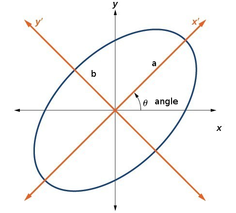
What are those sd* fields? According to the manual: The estimated standard deviations of the solution assuming a priori error model and error parameters by the positioning options. What it basically means is that the real GPS location will be located no further than three standard deviations across north and east from the measured location, most of (99.7%) the time. A way to represent this visually is to create an ellipse that maps this area of where the real location can be.

An ellipse can be uniquely defined from the lengths of the segments a and b and its rotation angle. For more details on how to get those ellipse parameters from the covariance matrix, please see the footnote.

Ground truth data

We also happen to have a file with the actual locations (also in longitudes and latitudes) of the object for the same time frame as the GPS (also in seconds), provided through another tracking method which is more accurate in this case.

This is because, the object was me running on a rooftop in Zürich wearing several tracking devices (not just GPS), and I knew exactly which floor tiles I was hitting.

The goal is to explore, visually, the relationship between the GPS data and the actual locations in time. I hope to get an idea of the accuracy, and what can influence it.

First look

Loading the GPS data into QGIS and Time Manager, we can indeed see the GPS locations vis-a-vis the actual locations in time.

Let’s see if the actual locations that were measured independently fall inside the ellipse coverage area. To do this, we need to use the covariance data to render ellipses.

Creating the ellipses

I considered using the ellipses marker from QGIS.

It is possible to switch from Millimeter to Map Unit and edit a data defined override for symbol width, height and rotation. Symbol width would be the a parameter of the ellipse, symbol height the b parameter and rotation simply the angle. The thing is, we haven’t computed any of these values yet, we just have the error covariance values in our dataset.

Because of the re-projections and matrix calculations inherent into extracting the a, b and angle of the error ellipse at each point in time, I decided to do this calculation offline using Python and relevant libraries, and then simply add a WKT text field with a polygon representation of the ellipse to the file I had. That way, the augmented data could be re-used outside QGIS, for example, to visualize using Leaflet or similar. I could have done a hybrid solution, where I calculated a, b and the angle offline, and then used the dynamic rendering capabilities of QGIS, as well.

I also decided to dump the csv into an sqlite database with an index on the time column, to make time range queries (which Time Manager does) run faster.

Putting it all together

The code for transforming the initial GPS data csv file into an sqlite database can be found in my github along with a small sample of the file containing the GPS data.

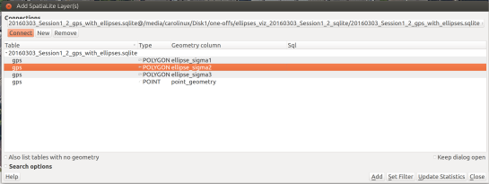
I created three ellipses per timestamp, to represent the three standard deviations. Opening QGIS (I used version: 2.12, Las Palmas) and going to Layer>Add Layer>Add SpatialLite Layer, we see the following dialog:

After adding the layer (say, for the second standard deviation ellipse), we can add it to Time Manager like so:

We do the process three times to add the three types of ellipses, taking care to style each ellipse differently. I used transparent fill for the second and third standard deviation ellipses.

I also added the data of my  actual positions.

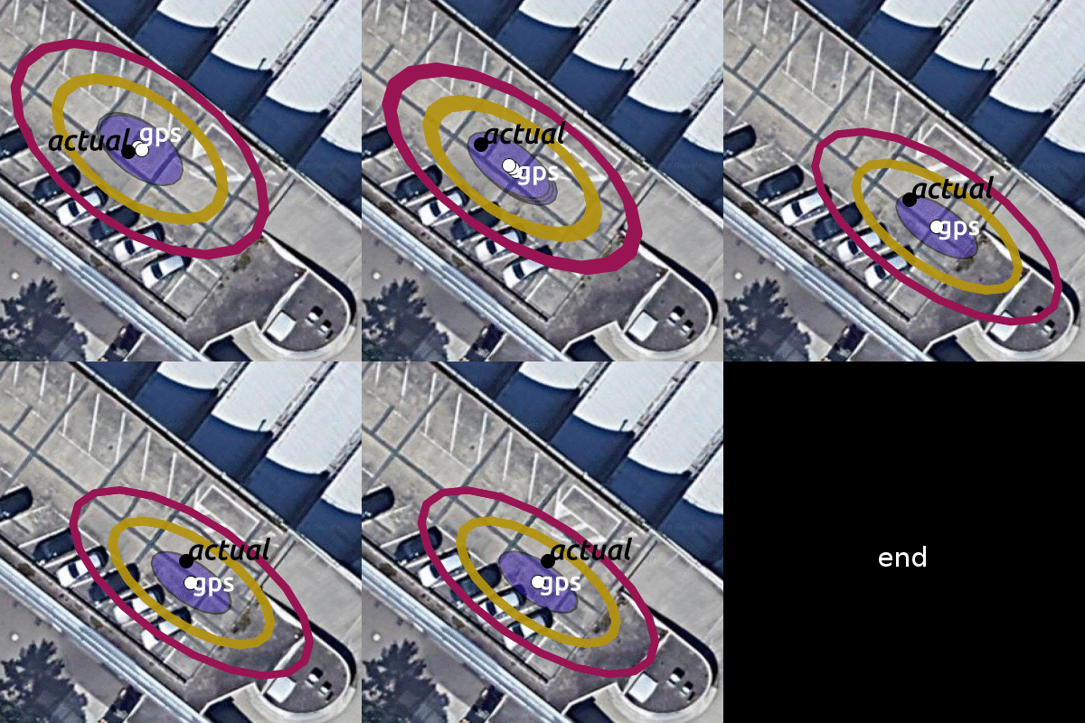
Here is an exported video of the trace (at a place in time where I go forward, backwards and forward again and then stay still).

Conclusions

Looking at the relationship between the actual data and the GPS data, we can see the following:

• Although the actual position differs from the measured one, the actual position always lies within one or two standard deviations of the measured position (so, inside the purple and golden ellipses).
• The direction of movement has greater uncertainty (the ellipse is elongated across the line I am running on).
• When I am standing still, the GPS position is still moving, and unfortunately does not converge to my actual stationary position, but drifts. More research is needed regarding what happens with the GPS data when the tracker is actually still.
• The GPS position doesn’t jump erratically, which can be good, however, it seems to have trouble ‘catching up’ with the actual position. This means if we’re looking to measure velocity in particular, the GPS tracker might underestimate that.

These findings are empirical, since they are extracted from a single visualization, but we have already learned some new things. We have some new ideas for what questions to ask on a large scale in the data, what additional experiments to run in the future and what limitations we may need to be aware of.

Thanks for reading!

Footnote: Error Covariance Matrix calculations

The error covariance matrix is (according to the definitions of the sd* columns in the manual):

It is not a diagonal matrix, which means that the errors across the ‘north’ dimension and the ‘east’ dimension, are not exactly independent.

An important detail is that, while the position is given in longitudes and latitudes, the sdn, sde and sdne fields are in meters. To address this in the code, we convert the longitude and latitudes using UTM projection, so that they are also in meters (northings and eastings).

For more details on the mathematics used to plot the ellipses check out this article by Robert Eisele and the implementation of the ellipse calculations on my github.

Do you sometimes start writing an SQL query and around at line 50 you get the feeling that it might be getting out of hand? If so, it might be useful to start breaking it down into smaller chunks and wrap those up into custom functions. Never done that? Don’t despair! There’s an excellent PL/pgSQL tutorial on postgresqltutorial.com to get you started.

To get an idea of the basic structure of a PL/pgSQL function and to proof that PostGIS datatypes work just fine in this context, here’s a basic function that takes a trajectory geometry and outputs its duration, i.e. the difference between its last and first timestamp:

CREATE OR REPLACE FUNCTION AG_Duration(traj geometry) 
RETURNS numeric LANGUAGE 'plpgsql'
AS $BODY$ 
BEGIN
RETURN ST_M(ST_EndPoint(traj))-ST_M(ST_StartPoint(traj));
END; $BODY$;

My end goal for this exercise was to implement a function that takes a trajectory and outputs the stops along this trajectory. Commonly, a stop is defined as a long stay within an area with a small radius. This leads us to the following definition:

CREATE OR REPLACE FUNCTION AG_DetectStops(
   traj geometry, 
   max_size numeric, 
   min_duration numeric)
RETURNS TABLE(sequence integer, geom geometry) 
-- implementation follows here!

Note how this function uses RETURNS TABLE to enable it to return all the stops that it finds. To add a line to the output table, we need to assign values to the sequence and geom variables and then use RETURN NEXT.

Another reason to use PL/pgSQL is that it enables us to write loops. And loops I wanted for my stop detection function! Specifically, I wanted to go through all the points in the trajectory:

FOR pt IN SELECT (ST_DumpPoints(traj)).geom LOOP
-- here comes the magic!
END LOOP;

Eventually the function should go through the trajectory and identify all segments that stay within an area with max_size diameter for at least min_duration time. To test for the area size, we can use:

IF ST_MaxDistance(segment,pt) <= max_size THEN is_stop := true; 

Putting everything together, my current implementation looks like this:

CREATE OR REPLACE FUNCTION AG_DetectStops(
   traj geometry,
   max_size numeric,
   min_duration numeric)
RETURNS TABLE(sequence integer, geom geometry) 
LANGUAGE 'plpgsql'
AS $BODY$
DECLARE 
   pt geometry;
   segment geometry;
   is_stop boolean;
   previously_stopped boolean;
   stop_sequence integer;
   p1 geometry;
BEGIN
segment := NULL;
sequence := 0;
is_stop := false;
previously_stopped := false;
p1 := NULL;
FOR pt IN SELECT (ST_DumpPoints(traj)).geom LOOP
   IF segment IS NULL AND p1 IS NULL THEN 
      p1 := pt; 
   ELSIF segment IS NULL THEN 
      segment := ST_MakeLine(p1,pt); 
      p1 := NULL;
      IF ST_Length(segment) <= max_size THEN is_stop := true; END IF; ELSE segment := ST_AddPoint(segment,pt); -- if we're in a stop, we want to grow the segment, otherwise we remove points to the specified min_duration IF NOT is_stop THEN WHILE ST_NPoints(segment) > 2 AND AG_Duration(ST_RemovePoint(segment,0)) >= min_duration LOOP
            segment := ST_RemovePoint(segment,0); 
         END LOOP;
      END IF;
      -- a stop is identified if the segment stays within a circle of diameter = max_size
      IF ST_Length(segment) <= max_size THEN is_stop := true; ELSIF ST_Distance(ST_StartPoint(segment),pt) > max_size THEN is_stop := false;
      ELSIF ST_MaxDistance(segment,pt) <= max_size THEN is_stop := true; ELSE is_stop := false; END IF; -- if we found the end of a stop, we need to check if it lasted long enough IF NOT is_stop AND previously_stopped THEN IF ST_M(ST_PointN(segment,ST_NPoints(segment)-1))-ST_M(ST_StartPoint(segment)) >= min_duration THEN
            geom := ST_RemovePoint(segment,ST_NPoints(segment)-1); 
            RETURN NEXT;
            sequence := sequence + 1;
            segment := NULL;
            p1 := pt;
         END IF;
      END IF;
   END IF;
   previously_stopped := is_stop;
END LOOP;
IF previously_stopped AND AG_Duration(segment) >= min_duration THEN 
   geom := segment; 
   RETURN NEXT; 
END IF;
END; $BODY$;

While this function is not really short, it’s so much more readable than my previous attempts of doing this in pure SQL. Some of the lines for determining is_stop are not strictly necessary but they do speed up processing.

Performance still isn’t quite where I’d like it to be. I suspect that all the adding and removing points from linestring geometries is not ideal. In general, it’s quicker to find shorter stops in smaller areas than longer stop in bigger areas.

Let’s test! 

Looking for a testing framework for PL/pgSQL, I found plpgunit on Github. While I did not end up using it, I did use its examples for inspiration to write a couple of tests, e.g.

CREATE OR REPLACE FUNCTION test.stop_at_beginning() RETURNS void LANGUAGE 'plpgsql'
AS $BODY$
DECLARE t0 integer; n0 integer;
BEGIN
WITH temp AS ( SELECT AG_DetectStops(
   ST_GeometryFromText('LinestringM(0 0 0, 0 0 1, 0.1 0.1 2, 2 2 3)'),
   1,1) stop 
)
SELECT ST_M(ST_StartPoint((stop).geom)), 
       ST_NPoints((stop).geom) FROM temp INTO t0, n0;	
IF t0 = 0 AND n0 = 3
   THEN RAISE INFO 'PASSED - Stop at the beginning of the trajectory';
   ELSE RAISE INFO 'FAILED - Stop at the beginning of the trajectory';
END IF;
END; $BODY$;

Basically, each test is yet another PL/pgSQL function that doesn’t return anything (i.e. returns void) but outputs messages about the status of the test. Here I made heavy use of the PERFORM statement which executes the provided function but discards the results:

Update: The source code for this function is now available on https://github.com/anitagraser/postgis-spatiotemporal

Last week, I traveled to Salzburg to attend the 30th AGIT conference and co-located English-speaking GI_Forum. Like in previous year, there were a lot of mobility and transportation research related presentations. Here are my personal highlights:

This year’s keynotes touched on a wide range of issues, from Sandeep Singhal (Google Cloud Storage) who – when I asked about the big table queries he showed – stated that they are not using a spatial index but are rather brute-forcing their way through massive data sets, to Laxmi Ramasubramanian @nycplanner (Hunter College City University of New York) who cautioned against tech arrogance and tendency to ignore expertise from other fields such as urban planning:

One issue that Laxmi particularly highlighted was the fact that many local communities are fighting excessive traffic caused by apps like Waze that suggest shortcuts through residential neighborhoods. Just because we can do something with (mobility) data, doesn’t necessarily mean that we should!

Not limited to mobility but very focused on open source, Jochen Albrecht (Hunter College City University of New York) invited the audience to join his quest for a spatial decision support system based on FOSS only at bit.ly/FiltersAndWeights and https://github.com/geojochen/fosssdss

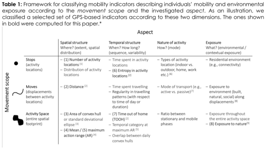
The session Spatial Perspectives on Healthy Mobility featured multiple interesting contributions, particularly by Michelle P. Fillekes who presented a framework of mobility indicators to assess daily mobility of study participants. It considers both spatial and temporal aspects of movement, as well as the movement context:

Figure from Michelle Pasquale Fillekes, Eleftheria Giannouli, Wiebren Zijlstra, Robert Weibel. Towards a Framework for Assessing Daily Mobility using GPS Data. DOI: 10.1553/giscience2018_01_s177 (under cc-by-nd)

It was also good to see that topics we’ve been working on in the past (popularity routing in this case) continue to be relevant and have been picked up in the German-speaking part of the conference:

Of course, I also presented some new work of my own, specifically my research into PostGIS trajectory datatypes which I’ve partially covered in a previous post on this blog and which is now published in Graser, A. (2018) Evaluating Spatio-temporal Data Models for Trajectories in PostGIS Databases. GI_Forum ‒ Journal of Geographic Information Science, 1-2018, 16-33. DOI: 10.1553/giscience2018_01_s16.

My introduction to GeoMesa talk failed to turn up any fellow Austrian GeoMesa users. So I’ll keep on looking and spreading the word. The most common question – and certainly no easy one at that – is how to determine the point where it becomes worth it to advance from regular databases to big data systems. It’s not just about the size of the data but also about how it is intended to be used. And of course, if you are one of those db admin whizzes who manages a distributed PostGIS setup in their sleep, you might be able to push the boundaries pretty far. On the other hand, if you already have some experience with the Hadoop ecosystem, getting started with tools like GeoMesa shouldn’t be too huge a step either. But that’s a topic for another day!

Since AGIT&GI_Forum are quite a big event with over 1,000 participants, it was not limited to movement data topics. You can find the first installment of English papers in GI_Forum 2018, Volume 1. As I understand it, there will be a second volume with more papers later this year.

This post is part of a series. Read more about movement data in GIS.