Related Plugins and Tags

QGIS Planet

Adding basemaps to PyQGIS maps in Jupyter notebooks

In the previous post, we investigated how to bring QGIS maps into Jupyter notebooks.

Today, we’ll take the next step and add basemaps to our maps. This is trickier than I would have expected. In particular, I was fighting with “invalid” OSM tile layers until I realized that my QGIS application instance somehow lacked the “WMS” provider.

In addition, getting basemaps to work also means that we have to take care of layer and project CRSes and on-the-fly reprojections. So let’s get to work:

from IPython.display import Image
from PyQt5.QtGui import QColor
from PyQt5.QtWidgets import QApplication
from qgis.core import QgsApplication, QgsVectorLayer, QgsProject, QgsRasterLayer, \
    QgsCoordinateReferenceSystem, QgsProviderRegistry, QgsSimpleMarkerSymbolLayerBase
from qgis.gui import QgsMapCanvas
app = QApplication([])
qgs = QgsApplication([], False)
qgs.setPrefixPath(r"C:\temp", True)  # setting a prefix path should enable the WMS provider
qgs.initQgis()
canvas = QgsMapCanvas()
project = QgsProject.instance()
map_crs = QgsCoordinateReferenceSystem('EPSG:3857')
canvas.setDestinationCrs(map_crs)
print("providers: ", QgsProviderRegistry.instance().providerList())

To add an OSM basemap, we use the xyz tiles option of the WMS provider:

urlWithParams = 'type=xyz&url=https://tile.openstreetmap.org/{z}/{x}/{y}.png&zmax=19&zmin=0&crs=EPSG3857'
rlayer = QgsRasterLayer(urlWithParams, 'OpenStreetMap', 'wms')  
print(rlayer.crs())
if rlayer.isValid():
    project.addMapLayer(rlayer)
else:
    print('invalid layer')
    print(rlayer.error().summary()) 

If there are issues with the WMS provider, rlayer.error().summary() should point them out.

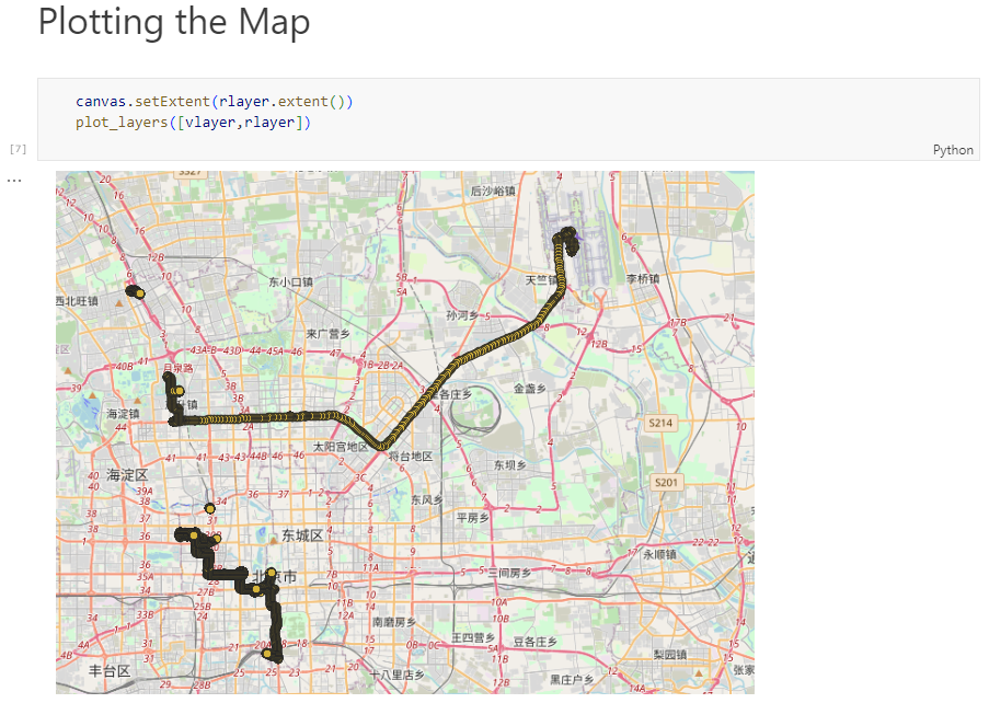
With both the vector layer and the basemap ready, we can finally plot the map:

canvas.setExtent(rlayer.extent())
plot_layers([vlayer,rlayer])

Of course, we can get more creative and style our vector layers:

vlayer.renderer().symbol().setColor(QColor("yellow"))
vlayer.renderer().symbol().symbolLayer(0).setShape(QgsSimpleMarkerSymbolLayerBase.Star)
vlayer.renderer().symbol().symbolLayer(0).setSize(10)
plot_layers([vlayer,rlayer])

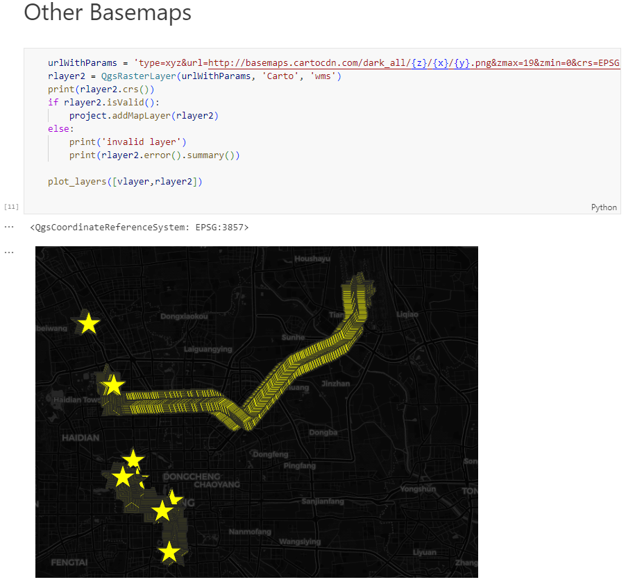
And to switch to other basemaps, we just need to update the URL accordingly, for example, to load Carto tiles instead:

urlWithParams = 'type=xyz&url=http://basemaps.cartocdn.com/dark_all/{z}/{x}/{y}.png&zmax=19&zmin=0&crs=EPSG3857'
rlayer2 = QgsRasterLayer(urlWithParams, 'Carto', 'wms')  
print(rlayer2.crs())
if rlayer2.isValid():
    project.addMapLayer(rlayer2)
else:
    print('invalid layer')
    print(rlayer2.error().summary()) 
    
plot_layers([vlayer,rlayer2])

You can find the whole notebook at: https://github.com/anitagraser/QGIS-resources/blob/master/qgis3/notebooks/basemaps.ipynb

Plotting large point CSV files quickly & interactively

Even with all their downsides, CSV files are still a common data exchange format – particularly between disciplines with different tech stacks. Indeed, “How to Specify Data Types of CSV Columns for Use in QGIS” (originally written in 2011) is still one of the most popular posts on this blog. QGIS continues to be quite handy for visualizing CSV file contents. However, there are times when it’s just not enough, particularly when the number of rows in the CSV is in the range of multiple million. The following example uses a 12 million point CSV:

To give you an idea of the waiting times in QGIS, I’ve run the following script which loads and renders the CSV:

from datetime import datetime

def get_time():
    t2 = datetime.now()
    print(t2)
    print(t2-t1)
    print('Done :)')

canvas = iface.mapCanvas()
canvas.mapCanvasRefreshed.connect(get_time)

print('Starting ...')

t0 = datetime.now()
print(t0)

print('Loading CSV ...')

uri = "file:///E:/Geodata/AISDK/raw_ais/aisdk_20170701.csv?type=csv&xField=Longitude&yField=Latitude&crs=EPSG:4326&"
vlayer = QgsVectorLayer(uri, "layer name you like", "delimitedtext")

t1 = datetime.now()
print(t1)
print(t1 - t0)

print('Rendering ...')

QgsProject.instance().addMapLayer(vlayer)

The script output shows that creating the vector layer takes 02:39 minutes and rendering it takes over 05:10 minutes:

Starting ...
2020-12-06 12:35:56.266002
Loading CSV ...
2020-12-06 12:38:35.565332
0:02:39.299330
Rendering ...
2020-12-06 12:43:45.637504
0:05:10.072172
Done :)

Rendered CSV file in QGIS

Panning and zooming around are no fun either since rendering takes so long. Changing from a single symbol renderer to, for example, a heatmap renderer does not improve the rendering times. So we need a different solutions when we want to efficiently explore large point CSV files.

The Pandas data analysis library is well-know for being a convenient tool for handling CSVs. However, it’s less clear how to use it as a replacement for desktop GIS for exploring large CSVs with point coordinates. My favorite solution so far uses hvPlot + HoloViews + Datashader to provide interactive Bokeh plots in Jupyter notebooks.

hvPlot provides a high-level plotting API built on HoloViews that provides a general and consistent API for plotting data in (Geo)Pandas, xarray, NetworkX, dask, and others. (Image source: https://hvplot.holoviz.org)

But first things first! Loading the CSV as a Pandas Dataframe takes 10.7 seconds. Pandas’ default plotting function (based on Matplotlib), however, takes around 13 seconds and only produces a static scatter plot.

Loading and plotting the CSV with Pandas

hvPlot to the rescue!

We only need two more steps to get faster and interactive map plots (plus background maps!): First, we need to reproject the lat/lon values. (There’s a warning here, most likely since some of the input lat/lon values are invalid.) Then, we replace plot() with hvplot() and voilà:

Plotting the CSV with Datashader

As you can see from the above GIF, the whole process barely takes 2 seconds and the resulting map plot is interactive and very responsive.

12 million points are far from the limit. As long as the Pandas DataFrame fits into memory, we are good and when the datasets get bigger than that, there are Dask DataFrames. But that’s a story for another day.

Movement data in GIS #30: synchronized trajectory animations with QGIS temporal controller

QGIS Temporal Controller is a powerful successor of TimeManager. Temporal Controller is a new core feature of the current development version and will be shipped with the 3.14 release. This post demonstrates two key advantages of this new temporal support:

  1. Expression support for defining start and end timestamps
  2. Integration into the PyQGIS API

These features come in very handy in many use cases. For example, they make it much easier to create animations from folders full of GPS tracks since the files can now be loaded and configured automatically:

Script & Temporal Controller in action (click for full resolution)

All tracks start at the same location but at different times. (Kudos for Andrew Fletcher for recordings these tracks and sharing them with me!) To create an animation that shows all tracks start simultaneously, we need to synchronize them. This synchronization can be achieved on-the-fly by subtracting the start time from all track timestamps using an expression:

directory = "E:/Google Drive/QGIS_Course/05_TimeManager/Example_Dayrides/"

def load_and_configure(filename):
    path = os.path.join(directory, filename)
    uri = 'file:///' + path + "?type=csv&escape=&useHeader=No&detectTypes=yes"
    uri = uri + "&crs=EPSG:4326&xField=field_3&yField=field_2"
    vlayer = QgsVectorLayer(uri, filename, "delimitedtext")
    QgsProject.instance().addMapLayer(vlayer)

    mode = QgsVectorLayerTemporalProperties.ModeFeatureDateTimeStartAndEndFromExpressions
    expression = """to_datetime(field_1) -
    make_interval(seconds:=minimum(epoch(to_datetime("field_1")))/1000)
    """

    tprops = vlayer.temporalProperties()
    tprops.setStartExpression(expression)
    tprops.setEndExpression(expression) # optional
    tprops.setMode(mode)
    tprops.setIsActive(True)

for filename in os.listdir(directory):
    if filename.endswith(".csv"):
        load_and_configure(filename)

The above script loads all CSV files from the given directory (field_1 is the timestamp, field_2 is y, and field_3 is x), enables sets the start and end expression as well as the corresponding temporal control mode and finally activates temporal rendering. The resulting config can be verified in the layer properties dialog:

To adapt this script to other datasets, it’s sufficient to change the file directory and revisit the layer uri definition as well as the field names referenced in the expression.


This post is part of a series. Read more about movement data in GIS.

Stand-alone PyQGIS scripts with OSGeo4W

PyQGIS scripts are great to automate spatial processing workflows. It’s easy to run these scripts inside QGIS but it can be even more convenient to run PyQGIS scripts without even having to launch QGIS. To create a so-called “stand-alone” PyQGIS script, there are a few things that need to be taken care of. The following steps show how to set up PyCharm for stand-alone PyQGIS development on Windows10 with OSGeo4W.

An essential first step is to ensure that all environment variables are set correctly. The most reliable approach is to go to C:\OSGeo4W64\bin (or wherever OSGeo4W is installed on your machine), make a copy of qgis-dev-g7.bat (or any other QGIS version that you have installed) and rename it to pycharm.bat:

Instead of launching QGIS, we want that pycharm.bat launches PyCharm. Therefore, we edit the final line in the .bat file to start pycharm64.exe:

In PyCharm itself, the main task to finish our setup is configuring the project interpreter:

First, we add a new “system interpreter” for Python 3.7 using the corresponding OSGeo4W Python installation.

To finish the interpreter config, we need to add two additional paths pointing to QGIS\python and QGIS\python\plugins:

That’s it! Now we can start developing our stand-alone PyQGIS script.

The following example shows the necessary steps, particularly:

  1. Initializing QGIS
  2. Initializing Processing
  3. Running a Processing algorithm
import sys

from qgis.core import QgsApplication, QgsProcessingFeedback
from qgis.analysis import QgsNativeAlgorithms

QgsApplication.setPrefixPath(r'C:\OSGeo4W64\apps\qgis-dev', True)
qgs = QgsApplication([], False)
qgs.initQgis()

# Add the path to processing so we can import it next
sys.path.append(r'C:\OSGeo4W64\apps\qgis-dev\python\plugins')
# Imports usually should be at the top of a script but this unconventional 
# order is necessary here because QGIS has to be initialized first
import processing
from processing.core.Processing import Processing

Processing.initialize()
QgsApplication.processingRegistry().addProvider(QgsNativeAlgorithms())
feedback = QgsProcessingFeedback()

rivers = r'D:\Documents\Geodata\NaturalEarthData\Natural_Earth_quick_start\10m_physical\ne_10m_rivers_lake_centerlines.shp'
output = r'D:\Documents\Geodata\temp\danube3.shp'
expression = "name LIKE '%Danube%'"

danube = processing.run(
    'native:extractbyexpression',
    {'INPUT': rivers, 'EXPRESSION': expression, 'OUTPUT': output},
    feedback=feedback
    )['OUTPUT']

print(danube)

PyQGIS101 part 10 published!

PyQGIS 101: Introduction to QGIS Python programming for non-programmers has now reached the part 10 milestone!

Beyond the obligatory Hello world! example, the contents so far include:

If you’ve been thinking about learning Python programming, but never got around to actually start doing it, give PyQGIS101 a try.

I’d like to thank everyone who has already provided feedback to the exercises. Every comment is important to help me understand the pain points of learning Python for QGIS.

I recently read an article – unfortunately I forgot to bookmark it and cannot locate it anymore – that described the problems with learning to program very well: in the beginning, it’s rather slow going, you don’t know the right terminology and therefore don’t know what to google for when you run into issues. But there comes this point, when you finally get it, when the terminology becomes clearer, when you start thinking “that might work” and it actually does! I hope that PyQGIS101 will be a help along the way.

PyQGIS for non-programmers

If you’re are following me on Twitter, you’ve certainly already read that I’m working on PyQGIS 101 a tutorial to help GIS users to get started with Python programming for QGIS.

I’ve often been asked to recommend Python tutorials for beginners and I’ve been surprised how difficult it can be to find an engaging tutorial for Python 3 that does not assume that the reader already knows all kinds of programming concepts.

It’s been a while since I started programming, but I do teach QGIS and Python programming for QGIS to university students and therefore have some ideas of which concepts are challenging. Nonetheless, it’s well possible that I overlook something that is not self explanatory. If you’re using PyQGIS 101 and find that some points could use further explanations, please leave a comment on the corresponding page.

PyQGIS 101 is a work in progress. I’d appreciate any feedback, particularly from beginners!

Porting Processing scripts to QGIS3

I’ll start with some tech talk first. Feel free to jump to the usage example further down if you are here for the edge bundling plugin.

As you certainly know, QGIS 3 brings a lot of improvements and under-the-hood changes. One of those changes affects all Python scripts. They need to be updated to Python 3 and the new PyQGIS API. (See the official migration guide for details.)

To get ready for the big 3.0 release, I’ve started porting my Processing tools. The edge bundling script is my first candidate for porting to QGIS 3. I also wanted to use this opportunity to “upgrade” from a simple script to a plugin that integrates into Processing.

I used Alexander Bruy’s “prepair for Processing” plugin as a template but you can also find an example template in your Processing folder. (On my system, it is located in C:\OSGeo4W64\apps\qgis-dev\python\plugins\processing\algs\exampleprovider.)

Since I didn’t want to miss the advantages of a good IDE, I set up PyCharm as described by Heikki Vesanto. This will give you code completion for Python 3 and PyQGIS which is very helpful for refactoring and porting. (I also tried Eclipse with PyDev but if you don’t have a favorite IDE yet, I find PyCharm easier to install and configure.)

My PyCharm startup script qgis3_pycharm.bat is a copy of C:\OSGeo4W64\bin\python-qgis-dev.bat with the last line altered to start PyCharm:

@echo off
call "%~dp0\o4w_env.bat"
call qt5_env.bat
call py3_env.bat
@echo off<span data-mce-type="bookmark" style="display: inline-block; width: 0px; overflow: hidden; line-height: 0;" class="mce_SELRES_start"></span>
path %OSGEO4W_ROOT%\apps\qgis-dev\bin;%PATH%
set QGIS_PREFIX_PATH=%OSGEO4W_ROOT:\=/%/apps/qgis-dev
set GDAL_FILENAME_IS_UTF8=YES
rem Set VSI cache to be used as buffer, see #6448
set VSI_CACHE=TRUE
set VSI_CACHE_SIZE=1000000
set QT_PLUGIN_PATH=%OSGEO4W_ROOT%\apps\qgis-dev\qtplugins;%OSGEO4W_ROOT%\apps\qt5\plugins
set PYTHONPATH=%OSGEO4W_ROOT%\apps\qgis-dev\python;%PYTHONPATH%
start /d "C:\Program Files\JetBrains\PyCharm\bin\" pycharm64.exe

In PyCharm File | Settings, I configured the OSGeo4W Python 3.6 interpreter and added qgis-dev and the plugin folder to its path:

With this setup done, we can go back to the code.

I first resolved all occurrences of import * in my script to follow good coding practices. For example:

from qgis.core import *

became

from qgis.core import QgsFeature, QgsPoint, QgsVector, QgsGeometry, QgsField, QGis<span data-mce-type="bookmark" style="display: inline-block; width: 0px; overflow: hidden; line-height: 0;" class="mce_SELRES_start"></span>

in this PR.

I didn’t even run the 2to3 script that is provided to make porting from Python 2 to Python 3 easier. Since the edge bundling code is mostly Numpy, there were almost no changes necessary. The only head scratching moment was when Numpy refused to add a map() return value to an array. So (with the help of Stackoverflow of course) I added a work around to convert the map() return value to an array as well:

flocal_x = map(forcecalcx, subtr_x, subtr_y, distance)
electrostaticforces_x[e_idx, :] += np.array(list(flocal_x))

The biggest change related to Processing is that the VectorWriter has been replaced by a QgsFeatureSink. It’s defined as a parameter of the edgebundling QgsProcessingAlgorithm:

self.addParameter(QgsProcessingParameterFeatureSink(
   self.OUTPUT,
   self.tr("Bundled edges"),
   QgsProcessing.TypeVectorLine)
)

And when the algorithm is run, the sink is filled with the output features:

(sink, dest_id) = self.parameterAsSink(
   parameters, self.OUTPUT, context,
   source.fields(), source.wkbType(), source.sourceCrs()
)

# code that creates features

sink.addFeature(feat, QgsFeatureSink.FastInsert)

The ported plugin is available on Github.

The edge bundling plugin in action

I haven’t uploaded the plugin to the official plugin repository yet, but you can already download if from Github and give it a try:

For this example, I’m using taxi pick-up and drop-off data provided by the NYC Taxi & Limousine Commission. I downloaded the January 2017 green taxi data and extracted all trips for the 1st of January. Then I created origin-destination (OD) lines using the QGIS virtual layer feature:

To get an interesting subset of the data, I extracted only those OD flows that cross the East River and have a count of at least 5 taxis:

Now the data is ready for bundling.

If you have installed the edge bundling plugin, the force-directed edge bundling algorithm should be available in the Processing toolbox. The UI of the edge bundling algorithm looks pretty much the same as it did for the QGIS 2 Processing script:

Since this is a small dataset with only 148 OD flows, the edge bundling processes is pretty quick and we can explore the results:

Beyond this core edge bundling algorithm, the repository also contains two more scripts that still need to be ported. They include dependencies on sklearn, so it will be interesting to see how straightforward it is to convert them.

Movement data in GIS #3: visualizing massive trajectory datasets

In the fist two parts of the Movement Data in GIS series, I discussed modeling trajectories as LinestringM features in PostGIS to overcome some common issues of movement data in GIS and presented a way to efficiently render speed changes along a trajectory in QGIS without having to split the trajectory into shorter segments.

While visualizing individual trajectories is important, the real challenge is trying to visualize massive trajectory datasets in a way that enables further analysis. The out-of-the-box functionality of GIS is painfully limited. Except for some transparency and heatmap approaches, there is not much that can be done to help interpret “hairballs” of trajectories. Luckily researchers in visual analytics have already put considerable effort into finding solutions for this visualization challenge. The approach I want to talk about today is by Andrienko, N., & Andrienko, G. (2011). Spatial generalization and aggregation of massive movement data. IEEE Transactions on visualization and computer graphics, 17(2), 205-219. and consists of the following main steps:

  1. Extracting characteristic points from the trajectories
  2. Grouping the extracted points by spatial proximity
  3. Computing group centroids and corresponding Voronoi cells
  4. Deviding trajectories into segments according to the Voronoi cells
  5. Counting transitions from one cell to another

The authors do a great job at describing the concepts and algorithms, which made it relatively straightforward to implement them in QGIS Processing. So far, I’ve implemented the basic logic but the paper contains further suggestions for improvements. This was also my first pyQGIS project that makes use of the measurement value support in the new geometry engine. The time information stored in the m-values is used to detect stop points, which – together with start, end, and turning points – make up the characteristic points of a trajectory.

The following animation illustrates the current state of the implementation: First the “hairball” of trajectories is rendered. Then we extract the characteristic points and group them by proximity. The big black dots are the resulting group centroids. From there, I skipped the Voronoi cells and directly counted transitions from “nearest to centroid A” to “nearest to centroid B”.

(data credits: GeoLife project)

From thousands of individual trajectories to a generalized representation of overall movement patterns (data credits: GeoLife project, map tiles: Stamen, map data: OSM)

The resulting visualization makes it possible to analyze flow strength as well as directionality. I have deliberately excluded all connections with a count below 10 transitions to reduce visual clutter. The cell size / distance between point groups – and therefore the level-of-detail – is one of the input parameters. In my example, I used a target cell size of approximately 2km. This setting results in connections which follow the major roads outside the city center very well. In the city center, where the road grid is tighter, trajectories on different roads mix and the connections are less clear.

Since trajectories in this dataset are not limited to car trips, it is expected to find additional movement that is not restricted to the road network. This is particularly noticeable in the dense area in the west where many slow trajectories – most likely from walking trips – are located. The paper also covers how to ensure that connections are limited to neighboring cells by densifying the trajectories before computing step 4.

trajectory_generalization

Running the scripts for over 18,000 trajectories requires patience. It would be worth evaluating if the first three steps can be run with only a subsample of the data without impacting the results in a negative way.

One thing I’m not satisfied with yet is the way to specify the target cell size. While it’s possible to measure ellipsoidal distances in meters using QgsDistanceArea (irrespective of the trajectory layer’s CRS), the initial regular grid used in step 2 in order to group the extracted points has to be specified in the trajectory layer’s CRS units – quite likely degrees. Instead, it may be best to transform everything into an equidistant projection before running any calculations.

It’s good to see that PyQGIS enables us to use the information encoded in PostGIS LinestringM features to perform spatio-temporal analysis. However, working with m or z values involves a lot of v2 geometry classes which work slightly differently than their v1 counterparts. It certainly takes some getting used to. This situation might get cleaned up as part of the QGIS 3 API refactoring effort. If you can, please support work on QGIS 3. Now is the time to shape the PyQGIS API for the following years!


Open source IDF router for QGIS

This is a follow-up on my previous post introducing an Open source IDF parser for QGIS. Today’s post takes the code further and adds routing functionality for foot, bike, and car routes including oneway streets and turn restrictions.

You can find the script in my QGIS-resources repository on Github. It creates an IDFRouter object based on an IDF file which you can use to compute routes.

The following screenshot shows an example car route in Vienna which gets quite complex due to driving restrictions. The dark blue line is computed by my script on GIP data while the light blue line is the route from OpenRouteService.org (via the OSM route plugin) on OSM data. Minor route geometry differences are due to slight differences in the network link geometries.

Screenshot 2015-08-01 16.29.57


Open source IDF parser for QGIS

IDF is the data format used by Austrian authorities to publish the official open government street graph. It’s basically a text file describing network nodes, links, and permissions for different modes of transport.

Since, to my knowledge, there hasn’t been any open source IDF parser available so far, I’ve started to write my own using PyQGIS. You can find the script which is meant to be run in the QGIS Python console in my Github QGIS-resources repo.

I haven’t implemented all details yet but it successfully parses nodes and links from the two example IDF files that have been published so far as can be seen in the following screenshot which shows the Klagenfurt example data:

Screenshot 2015-07-23 16.23.25

If you are interested in advancing this project, just get in touch here or on Github.


Game of Life – Raster edition

You probably remember my Game of Life posts from last year: Experiments with Conway’s Game of Life & More experiments with Game of Life where I developed a vector-based version of GoL.

Richard Wen and Claus Rinner at Ryerson University now published a raster-based version.

Here’s a screenshot of the script in action:

Screenshot 2015-03-08 20.04.07

The code is hosted on Github and I’m sure there will be many other ideas which can build on code snippets to read and write raster cell values.

For more info, please visit the GIS at Ryerson blog.


More experiments with Game of Life

As promised in my recent post “Experiments with Conway’s Game of Life”, I have been been looking into how to improve my first implementation. The new version which you can now find on Github is fully contained in one Python script which runs in the QGIS console. Additionally, the repository contains a CSV with the grid definition for a Gosper glider gun and the layer style QML.

Rather than creating a new Shapefile for each iteration like in the first implementation, this script uses memory layers to save the game status.

You can see it all in action in the following video:

(video available in HD)

Thanks a lot to Nathan Woodrow for the support in getting the animation running!

Sometimes there are still hick-ups causing steps to be skipped but overall it is running nicely now. Another approach would be to change the layer attributes rather than creating more and more layers but I like to be able to go through all the resulting layers after they have been computed.


Experiments with Conway’s Game of Life

This experiment is motivated by a discussion I had with Dr. Claus Rinner about introducing students to GIS concepts using Conway’s Game of Life. Conway’s Game of Life is a popular example to demonstrate cellular automata. Based on an input grid of “alive” and “dead” cells, new cell values are computed on each iteration based on four simple rules for the cell and its 8 neighbors:

  1. Any live cell with fewer than two live neighbours dies, as if caused by under-population.
  2. Any live cell with two or three live neighbours lives on to the next generation.
  3. Any live cell with more than three live neighbours dies, as if by overcrowding.
  4. Any dead cell with exactly three live neighbours becomes a live cell, as if by reproduction.

(Source: Wikipedia – Conway’s Game of Life)

Based on these simple rules, effects like the following “glider gun” can be achieved:

Gospers glider gun.gif
Gospers glider gun” by KieffOwn work. Licensed under CC BY-SA 3.0 via Wikimedia Commons.

There are some Game of Life implementations for GIS out there, e.g. scripts for ArcGIS or a module for SAGA. Both of these examples are raster-based. Since I couldn’t find any examples of raster manipulation like this in pyQGIS, I decided to instead implement a vector version: a Processing script which receives an input grid of cells and outputs the next iteration based on the rules of Game of Life. In the following screencast, you can see the Processing script being called repeatedly by a script from the Python console:

So far, it’s a quick and dirty first implementation. To make it more smooth, I’m considering adding spatial indexing and using memory layers instead of having Processing create a bunch of Shapefiles.

It would also be interesting to see a raster version done in PyQGIS. Please leave a comment if you have any ideas how this could be achieved.


A routing script for the Processing toolbox

Did you know that there is a network analysis library in QGIS core? It’s well hidden so far, but at least it’s documented in the PyQGIS Cookbook. The code samples from the cookbook can be used in the QGIS Python console and you can play around to get a grip of what the different steps are doing.

As a first exercise, I’ve decided to write a Processing script which will use the network analysis library to create a network-based route layer from a point layer input. You can find the result on Github.

You can get a Spatialite file with testdata from Github as well. It contains a network and a routepoints1 layer:

points_to_route1

The interface of the points_to_route tool is very simple. All it needs as an input is information about which layer should be used as a network and which layer contains the route points:

points_to_route0

The input points are considered to be ordered. The tool always routes between consecutive points.

The result is a line layer with one line feature for each point pair:

points_to_route2

The network analysis library is a really great new feature and I hope we will see a lot of tools built on top of it.


How to Install Sphinx

This post summarizes how to install sphinx on Windows to contribute to PyQGIS Cookbook. I’m writing this as I go, so this most likely won’t be perfect.

I used my Python 2.6 stand-alone installation (not the one in OSGeo4W).

  1. Get the Sphinx egg from http://pypi.python.org/pypi/Sphinx
  2. If you don’t have it, install setuptools to get the easy_install script http://pypi.python.org/pypi/setuptools
  3. In C:\Python26\Scripts run easy_install -U sphinx
  4. Get the PyQGIS source from https://github.com/qgis/QGIS-Developer-Cookbook
  5. Create a build folder inside the QGIS-Developer-Cookbook
  6. Now you can build the Cookbook: sphinx-build "C:\Users\Anita\QGIS\QGIS-Developer-Cookbook\source" "C:\Users\Anita\QGIS\QGIS-Developer-Cookbook\build"

The build folder should now contain the Cookbook .html files.


How to Add a Legend to Your PyQGIS Application

In his post “Layer list widget for PyQGIS applications”, German Carrillo describes how to add a legend to your own PyQGIS application. You get to download the source code for the legend widget to include into your project.


Back to Top

Sustaining Members