Related Plugins and Tags

QGIS Planet

Dashboards in QGIS

If you are following QGIS topics on social media, you may have already seen this but if you don’t, I recommend having a look at Tim Sutton’s most recent adventures in building dashboards with QGIS:

The dashboard is built using labeling and geometry generator functionality. This means that they work in the QGIS application map window as well as in layouts. As hinted at in the screenshot above, the dashboard can show information about whole layers as well as interactive selections.

Here’s a full walk-through Tim published yesterday:

You can follow the further development via Tim’s tweets or the dedicated Github issue (where you can even find an example QGIS dashboard project in a GeoPacakge for download).

More icons & symbols for QGIS – updated

The 2016 post More icons & symbols for QGIS still regularly makes it to the top 10 list of posts by visitors. I wouldn’t attribute this popularity to the quality of this particular post, however. Instead, it’s a pretty clear sign that QGIS users are actively searching for more styling resources to add to their installations.

When it comes to styling resources, the person to follow right now is clearly Klas Karlsson who’s been keeping a steady stream of styling-related posts coming to Twitter:

Additionally, he’s the master-mind behind QGIS Hub, a – currently prototypical – platform for sharing styling resources and print layout templates:

If you are interested in sharing styling resources, head over there. Similarly, if you want to lend a hand developing QGIS Hub, get in touch!

Movement data in GIS #30: synchronized trajectory animations with QGIS temporal controller

QGIS Temporal Controller is a powerful successor of TimeManager. Temporal Controller is a new core feature of the current development version and will be shipped with the 3.14 release. This post demonstrates two key advantages of this new temporal support:

  1. Expression support for defining start and end timestamps
  2. Integration into the PyQGIS API

These features come in very handy in many use cases. For example, they make it much easier to create animations from folders full of GPS tracks since the files can now be loaded and configured automatically:

Script & Temporal Controller in action (click for full resolution)

All tracks start at the same location but at different times. (Kudos for Andrew Fletcher for recordings these tracks and sharing them with me!) To create an animation that shows all tracks start simultaneously, we need to synchronize them. This synchronization can be achieved on-the-fly by subtracting the start time from all track timestamps using an expression:

directory = "E:/Google Drive/QGIS_Course/05_TimeManager/Example_Dayrides/"

def load_and_configure(filename):
    path = os.path.join(directory, filename)
    uri = 'file:///' + path + "?type=csv&escape=&useHeader=No&detectTypes=yes"
    uri = uri + "&crs=EPSG:4326&xField=field_3&yField=field_2"
    vlayer = QgsVectorLayer(uri, filename, "delimitedtext")
    QgsProject.instance().addMapLayer(vlayer)

    mode = QgsVectorLayerTemporalProperties.ModeFeatureDateTimeStartAndEndFromExpressions
    expression = """to_datetime(field_1) -
    make_interval(seconds:=minimum(epoch(to_datetime("field_1")))/1000)
    """

    tprops = vlayer.temporalProperties()
    tprops.setStartExpression(expression)
    tprops.setEndExpression(expression) # optional
    tprops.setMode(mode)
    tprops.setIsActive(True)

for filename in os.listdir(directory):
    if filename.endswith(".csv"):
        load_and_configure(filename)

The above script loads all CSV files from the given directory (field_1 is the timestamp, field_2 is y, and field_3 is x), enables sets the start and end expression as well as the corresponding temporal control mode and finally activates temporal rendering. The resulting config can be verified in the layer properties dialog:

To adapt this script to other datasets, it’s sufficient to change the file directory and revisit the layer uri definition as well as the field names referenced in the expression.


This post is part of a series. Read more about movement data in GIS.

TimeManager is dead, long live the Temporal Controller!

TimeManager turns 10 this year. The code base has made the transition from QGIS 1.x to 2.x and now 3.x and it would be wrong to say that it doesn’t show ;-)

Now, it looks like the days of TimeManager are numbered. Four days ago, Nyall Dawson has added native temporal support for vector layers to QGIS. This is part of a larger effort of adding time support for rasters, meshes, and now also vectors.

The new Temporal Controller panel looks similar to TimeManager. Layers are configured through the new Temporal tab in Layer Properties. The temporal dimension can be used in expressions to create fancy time-dependent styles:

temporal1

TimeManager Geolife demo converted to Temporal Controller (click for full resolution)

Obviously, this feature is brand new and will require polishing. Known issues listed by Nyall include limitations of supported time fields (only fields with datetime type are supported right now, strings cannot be used) and worse performance than TimeManager since features are filtered in QGIS rather than in the backend.

If you want to give the new Temporal Controller a try, you need to install the current development version, e.g. qgis-dev in OSGeo4W.


Update from May 16:

Many of the limitations above have already been addressed.

Last night, Nyall has recorded a one hour tutorial on this new feature, enjoy:

QGIS video tutorials: election maps, hydrology, and more

Mapping spatial decision patterns, such as election results, is always a hot topic. That’s why we decided to include a recipe for election maps in our QGIS Map Design books. What’s new is that this recipe is now available as a free video tutorial recorded by Oliver Burdekin:

This video is just one of many recently published video tutorials that have been created by QGIS community members.

For example, Hans van der Kwast and Kurt Menke have recorded a 7-part series on QGIS for Hydrological Applications:

and Klas Karlsson’s Youtube channel is also always worth a follow:

For the Pythonically inclined among you, there is also a new version of Python in QGIS on the Automating GIS-processes channel:


Five QGIS network analysis toolboxes for routing and isochrones

In the past, network analysis capabilities in QGIS were rather limited or not straight-forward to use. This has changed! In QGIS 3.x, we now have a wide range of network analysis tools, both for use case where you want to use your own network data, as well as use cases where you don’t have access to appropriate data or just prefer to use an existing service.

This blog post aims to provide an overview of the options:

  1. Based on local network data
    1. Default QGIS Processing network analysis tools
    2. QNEAT3 plugin
  2. Based on web services
    1. Hqgis plugin (HERE)
    2. ORS Tools plugin (openrouteservice.org)
    3. TravelTime platform plugin (TravelTime platform)

All five options provide Processing toolbox integration but not at the same level.

If you are a regular reader of this blog, you’re probably also aware of the pgRoutingLayer plugin. However, I’m not including it in this list due to its dependency on PostGIS and its pgRouting extension.

Processing network analysis tools

The default Processing network analysis tools are provided out of the box. They provide functionality to compute least cost paths and service areas (distance or time) based on your own network data. Inputs can be individual points or layers of points:

The service area tools return reachable edges and / or nodes rather than a service area polygon:

QNEAT3 plugin

The QNEAT3 (short for Qgis Network Analysis Toolbox 3) Plugin aims to provide sophisticated QGIS Processing-Toolbox algorithms in the field of network analysis. QNEAT3 is integrated in the QGIS3 Processing Framework. It offers algorithms that range from simple shortest path solving to more complex tasks like Iso-Area (aka service areas, accessibility polygons) and OD-Matrix (Origin-Destination-Matrix) computation.

QNEAT3 is an alternative for use case where you want to use your own network data.

For more details see the QNEAT3 documentation at: https://root676.github.io/index.html

Hqgis plugin

Access the HERE API from inside QGIS using your own HERE-API key. Currently supports Geocoding, Routing, POI-search and isochrone analysis.

Hqgis currently does not expose all its functionality to the Processing toolbox:

Instead, the full set of functionality is provided through the plugin GUI:

This plugin requires a HERE API key.

ORS Tools plugin

ORS Tools provides access to most of the functions of openrouteservice.org, based on OpenStreetMap. The tool set includes routing, isochrones and matrix calculations, either interactive in the map canvas or from point files within the processing framework. Extensive attributes are set for output files, incl. duration, length and start/end locations.

ORS Tools is based on OSM data. However, using this plugin still requires an openrouteservice.org API key.

TravelTime platform plugin

This plugin adds a toolbar and processing algorithms allowing to query the TravelTime platform API directly from QGIS. The TravelTime platform API allows to obtain polygons based on actual travel time using several transport modes rather, allowing for much more accurate results than simple distance calculations.

The TravelTime platform plugin requires a TravelTime platform API key.

For more details see: https://blog.traveltimeplatform.com/isochrone-qgis-plugin-traveltime

Stand-alone PyQGIS scripts with OSGeo4W

PyQGIS scripts are great to automate spatial processing workflows. It’s easy to run these scripts inside QGIS but it can be even more convenient to run PyQGIS scripts without even having to launch QGIS. To create a so-called “stand-alone” PyQGIS script, there are a few things that need to be taken care of. The following steps show how to set up PyCharm for stand-alone PyQGIS development on Windows10 with OSGeo4W.

An essential first step is to ensure that all environment variables are set correctly. The most reliable approach is to go to C:\OSGeo4W64\bin (or wherever OSGeo4W is installed on your machine), make a copy of qgis-dev-g7.bat (or any other QGIS version that you have installed) and rename it to pycharm.bat:

Instead of launching QGIS, we want that pycharm.bat launches PyCharm. Therefore, we edit the final line in the .bat file to start pycharm64.exe:

In PyCharm itself, the main task to finish our setup is configuring the project interpreter:

First, we add a new “system interpreter” for Python 3.7 using the corresponding OSGeo4W Python installation.

To finish the interpreter config, we need to add two additional paths pointing to QGIS\python and QGIS\python\plugins:

That’s it! Now we can start developing our stand-alone PyQGIS script.

The following example shows the necessary steps, particularly:

  1. Initializing QGIS
  2. Initializing Processing
  3. Running a Processing algorithm
import sys

from qgis.core import QgsApplication, QgsProcessingFeedback
from qgis.analysis import QgsNativeAlgorithms

QgsApplication.setPrefixPath(r'C:\OSGeo4W64\apps\qgis-dev', True)
qgs = QgsApplication([], False)
qgs.initQgis()

# Add the path to processing so we can import it next
sys.path.append(r'C:\OSGeo4W64\apps\qgis-dev\python\plugins')
# Imports usually should be at the top of a script but this unconventional 
# order is necessary here because QGIS has to be initialized first
import processing
from processing.core.Processing import Processing

Processing.initialize()
QgsApplication.processingRegistry().addProvider(QgsNativeAlgorithms())
feedback = QgsProcessingFeedback()

rivers = r'D:\Documents\Geodata\NaturalEarthData\Natural_Earth_quick_start\10m_physical\ne_10m_rivers_lake_centerlines.shp'
output = r'D:\Documents\Geodata\temp\danube3.shp'
expression = "name LIKE '%Danube%'"

danube = processing.run(
    'native:extractbyexpression',
    {'INPUT': rivers, 'EXPRESSION': expression, 'OUTPUT': output},
    feedback=feedback
    )['OUTPUT']

print(danube)

Easy Processing scripts comeback in QGIS 3.6

When QGIS 3.0 was release, I published a Processing script template for QGIS3. While the script template is nicely pythonic, it’s also pretty long and daunting for non-programmers. This fact didn’t go unnoticed and Nathan Woodrow in particular started to work on a QGIS enhancement proposal to improve the situation and make writing Processing scripts easier, while – at the same time – keeping in line with common Python styles.

While the previous template had 57 lines of code, the new template only has 26 lines – 50% less code, same functionality! (Actually, this template provides more functionality since it also tracks progress and ensures that the algorithm can be cancelled.)

from qgis.processing import alg
from qgis.core import QgsFeature, QgsFeatureSink

@alg(name="ex_new", label=alg.tr("Example script (new style)"), group="examplescripts", group_label=alg.tr("Example Scripts"))
@alg.input(type=alg.SOURCE, name="INPUT", label="Input layer")
@alg.input(type=alg.SINK, name="OUTPUT", label="Output layer")
def testalg(instance, parameters, context, feedback, inputs):
    """
    Description goes here. (Don't delete this! Removing this comment will cause errors.)
    """
    source = instance.parameterAsSource(parameters, "INPUT", context)

    (sink, dest_id) = instance.parameterAsSink(
        parameters, "OUTPUT", context,
        source.fields(), source.wkbType(), source.sourceCrs())

    total = 100.0 / source.featureCount() if source.featureCount() else 0
    features = source.getFeatures()
    for current, feature in enumerate(features):
        if feedback.isCanceled():
            break
        out_feature = QgsFeature(feature)
        sink.addFeature(out_feature, QgsFeatureSink.FastInsert)
        feedback.setProgress(int(current * total))

    return {"OUTPUT": dest_id}

The key improvement are the new decorators that turn an ordinary function (such as testalg in the template) into a Processing algorithm. Decorators start with @ and are written above a function definition. The @alg decorator declares that the following function is a Processing algorithm, defines its name and assigns it to an algorithm group. The @alg.input decorator creates an input parameter for the algorithm. Similarly, there is a @alg.output decorator for output parameters.

For a longer example script, check out the original QGIS enhancement proposal thread!

For now, this new way of writing Processing scripts is only supported by QGIS 3.6 but there are plans to back-port this improvement to 3.4 once it is more mature. So give it a try and report back!

Movement data in GIS #20: Trajectools v1 released!

In previous posts, I already wrote about Trajectools and some of the functionality it provides to QGIS Processing including:

There are also tools to compute heading and speed which I only talked about on Twitter.

Trajectools is now available from the QGIS plugin repository.

The plugin includes sample data from MarineCadastre downloads and the Geolife project.

Under the hood, Trajectools depends on GeoPandas!

If you are on Windows, here’s how to install GeoPandas for OSGeo4W:

  1. OSGeo4W installer: install python3-pip
  2. Environment variables: add GDAL_VERSION = 2.3.2 (or whichever version your OSGeo4W installation currently includes)
  3. OSGeo4W shell: call C:\OSGeo4W64\bin\py3_env.bat
  4. OSGeo4W shell: pip3 install geopandas (this will error at fiona)
  5. From https://www.lfd.uci.edu/~gohlke/pythonlibs/#fiona: download Fiona-1.7.13-cp37-cp37m-win_amd64.whl
  6. OSGeo4W shell: pip3 install path-to-download\Fiona-1.7.13-cp37-cp37m-win_amd64.whl
  7. OSGeo4W shell: pip3 install geopandas
  8. (optionally) From https://www.lfd.uci.edu/~gohlke/pythonlibs/#rtree: download Rtree-0.8.3-cp37-cp37m-win_amd64.whl and pip3 install it

If you want to use this functionality outside of QGIS, head over to my movingpandas project!

Movement data in GIS #19: splitting trajectories by date

Many current movement data sources provide more or less continuous streams of object locations. For example, the AIS system provides continuous locations of vessels (mostly ships). This continuous stream of locations – let’s call it track – starts when we first record the vessel and ends with the last record. This start and end does not necessarily coincide with the start or end of a vessel voyage from one port to another. The stream start and end do not have any particular meaning. Instead, if we want to see what’s going on, we need to split the track into meaningful segments. One such segmentation – albeit a simple one – is to split tracks by day. This segmentation assumes that day/night changes affect the movement of our observed object. For many types of objects – those who mostly stay still during the night – this will work reasonably well.

For example, the following screenshot shows raw data of one particular vessel in the Boston region. By default, QGIS provides a Points to Path to convert points to lines. This tool takes one “group by” and one “order by” field. Therefore, if we want one trajectory per ship per day, we’d first have to create a new field that combines ship ID and day so that we can use this combination as a “group by” field. Additionally, the resulting lines loose all temporal information.

To simplify this workflow, Trajectools now provides a new algorithm that creates day trajectories and outputs LinestringM features. Using the Day trajectories from point layer tool, we can immediately see that our vessel of interest has been active for three consecutive days: entering our observation area on Nov 5th, moving to Boston where it stayed over night, then moving south to Weymouth on the next day, and leaving on the 7th.

Since the resulting trajectories are LinestringM features with time information stored in the M value, we can also visualize the speed of movement (as discussed in part #2 of this series):

Flow maps in QGIS – no plugins needed!

If you’ve been following my posts, you’ll no doubt have seen quite a few flow maps on this blog. This tutorial brings together many different elements to show you exactly how to create a flow map from scratch. It’s the result of a collaboration with Hans-Jörg Stark from Switzerland who collected the data.

The flow data

The data presented in this post stems from a survey conducted among public transport users, especially commuters (available online at: https://de.surveymonkey.com/r/57D33V6). Among other questions, the questionnair asks where the commuters start their journey and where they are heading.

The answers had to be cleaned up to correct for different spellings, spelling errors, and multiple locations in one field. This cleaning and the following geocoding step were implemented in Python. Afterwards, the flow information was aggregated to count the number of nominations of each connection between different places. Finally, these connections (edges that contain start id, destination id and number of nominations) were stored in a text file. In addition, the locations were stored in a second text file containing id, location name, and co-ordinates.

Why was this data collected?

Besides travel demand, Hans-Jörg’s survey also asks participants about their coffee consumption during train rides. Here’s how he tells the story behind the data:

As a nearly daily commuter I like to enjoy a hot coffee on my train rides. But what has bugged me for a long time is the fact the coffee or hot beverages in general are almost always served in a non-reusable, “one-use-only-and-then-throw-away” cup. So I ended up buying one of these mostly ugly and space-consuming reusable cups. Neither system seem to satisfy me as customer: the paper-cup produces a lot of waste, though it is convenient because I carry it only when I need it. With the re-usable cup I carry it all day even though most of the time it is empty and it is clumsy and consumes the limited space in bag.

So I have been looking for a system that gets rid of the disadvantages or rather provides the advantages of both approaches and I came up with the following idea: Installing a system that provides a re-usable cup that I only have with me when I need it.

In order to evaluate the potential for such a system – which would not only imply a material change of the cups in terms of hardware but also introduce some software solution with the convenience of getting back the necessary deposit that I pay as a customer and some software-solution in the back-end that handles all the cleaning, distribution to the different coffee-shops and managing a balanced stocking in the stations – I conducted a survey

The next step was the geographic visualization of the flow data and this is where QGIS comes into play.

The flow map

Survey data like the one described above is a common input for flow maps. There’s usually a point layer (here: “nodes”) that provides geographic information and a non-spatial layer (here: “edges”) that contains the information about the strength or weight of a flow between two specific nodes:

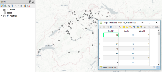
The first step therefore is to create the flow line features from the nodes and edges layers. To achieve our goal, we need to join both layers. Sounds like a job for SQL!

More specifically, this is a job for Virtual Layers: Layer | Add Layer | Add/Edit Virtual Layer

SELECT StartID, DestID, Weight, 
       make_line(a.geometry, b.geometry)
FROM edges
JOIN nodes a ON edges.StartID = a.ID
JOIN nodes b ON edges.DestID = b.ID
WHERE a.ID != b.ID 

This SQL query joins the geographic information from the nodes table to the flow weights in the edges table based on the node IDs. In the last line, there is a check that start and end node ID should be different in order to avoid zero-length lines.

By styling the resulting flow lines using data-driven line width and adding in some feature blending, it’s possible to create some half decent maps:

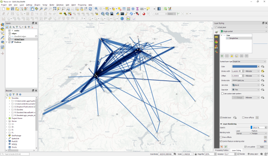
However, we can definitely do better. Let’s throw in some curved arrows!

The arrow symbol layer type automatically creates curved arrows if the underlying line feature has three nodes that are not aligned on a straight line.

Therefore, to turn our straight lines into curved arrows, we need to add a third point to the line feature and it has to have an offset. This can be achieved using a geometry generator and the offset_curve() function:

make_line(
   start_point($geometry),
   centroid(
      offset_curve(
         $geometry, 
         length($geometry)/-5.0
      )
   ),
   end_point($geometry)
)

Additionally, to achieve the effect described in New style: flow map arrows, we extend the geometry generator to crop the lines at the beginning and end:

difference(
   difference(
      make_line(
         start_point($geometry),
         centroid(
            offset_curve(
               $geometry, 
               length($geometry)/-5.0
            )
         ),
	 end_point($geometry)
      ),
      buffer(start_point($geometry), 0.01)
   ),
   buffer(end_point( $geometry), 0.01)
)

By applying data-driven arrow and arrow head sizes, we can transform the plain flow map above into a much more appealing map:

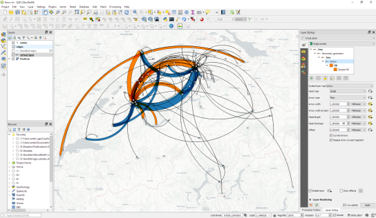
The two different arrow colors are another way to emphasize flow direction. In this case, orange arrows mark flows to the west, while blue flows point east.

CASE WHEN
 x(start_point($geometry)) - x(end_point($geometry)) < 0
THEN
 '#1f78b4'
ELSE
 '#ff7f00'
END

Conclusion

As you can see, virtual layers and geometry generators are a powerful combination. If you encounter performance problems with the virtual layer, it’s always possible to make it permanent by exporting it to a file. This will speed up any further visualization or analysis steps.

PyQGIS101 part 10 published!

PyQGIS 101: Introduction to QGIS Python programming for non-programmers has now reached the part 10 milestone!

Beyond the obligatory Hello world! example, the contents so far include:

If you’ve been thinking about learning Python programming, but never got around to actually start doing it, give PyQGIS101 a try.

I’d like to thank everyone who has already provided feedback to the exercises. Every comment is important to help me understand the pain points of learning Python for QGIS.

I recently read an article – unfortunately I forgot to bookmark it and cannot locate it anymore – that described the problems with learning to program very well: in the beginning, it’s rather slow going, you don’t know the right terminology and therefore don’t know what to google for when you run into issues. But there comes this point, when you finally get it, when the terminology becomes clearer, when you start thinking “that might work” and it actually does! I hope that PyQGIS101 will be a help along the way.

Movement data in GIS #17: spatial analysis of GeoPandas trajectories

In Movement data in GIS #16, I presented a new way to deal with trajectory data using GeoPandas and how to load the trajectory GeoDataframes as a QGIS layer. Following up on this initial experiment, I’ve now implemented a first version of an algorithm that performs a spatial analysis on my GeoPandas trajectories.

The first spatial analysis algorithm I’ve implemented is Clip trajectories by extent. Implementing this algorithm revealed a couple of pitfalls:

  • To achieve correct results, we need to compute spatial intersections between linear trajectory segments and the extent. Therefore, we need to convert our point GeoDataframe to a line GeoDataframe.
  • Based on the spatial intersection, we need to take care of computing the corresponding timestamps of the events when trajectories enter or leave the extent.
  • A trajectory can intersect the extent multiple times. Therefore, we cannot simply use the global minimum and maximum timestamp of intersecting segments.
  • GeoPandas provides spatial intersection functionality but if the trajectory contains consecutive rows without location change, these will result in zero length lines and those cause an empty intersection result.

So far, the clip result only contains the trajectory id plus a suffix indicating the sequence of the intersection segments for a specific trajectory (because one trajectory can intersect the extent multiple times). The following screenshot shows one highlighted trajectory that intersects the extent three times and the resulting clipped trajectories:

This algorithm together with the basic trajectory from points algorithm is now available in a Processing algorithm provider plugin called Processing Trajectory.

Note: This plugin depends on GeoPandas.

Note for Windows users: GeoPandas is not a standard package that is available in OSGeo4W, so you’ll have to install it manually. (For the necessary steps, see this answer on gis.stackexchange.com)

The implemented tests show how to use the Trajectory class independently of QGIS. So far, I’m only testing the spatial properties though:

def test_two_intersections_with_same_polygon(self):
    polygon = Polygon([(5,-5),(7,-5),(7,12),(5,12),(5,-5)])
    data = [{'id':1, 'geometry':Point(0,0), 't':datetime(2018,1,1,12,0,0)},
        {'id':1, 'geometry':Point(6,0), 't':datetime(2018,1,1,12,10,0)},
        {'id':1, 'geometry':Point(10,0), 't':datetime(2018,1,1,12,15,0)},
        {'id':1, 'geometry':Point(10,10), 't':datetime(2018,1,1,12,30,0)},
        {'id':1, 'geometry':Point(0,10), 't':datetime(2018,1,1,13,0,0)}]
    df = pd.DataFrame(data).set_index('t')
    geo_df = GeoDataFrame(df, crs={'init': '31256'})
    traj = Trajectory(1, geo_df)
    intersections = traj.intersection(polygon)
    result = []
    for x in intersections:
        result.append(x.to_linestring())
    expected_result = [LineString([(5,0),(6,0),(7,0)]), LineString([(7,10),(5,10)])]
    self.assertEqual(result, expected_result) 

One issue with implementing the algorithms as QGIS Processing tools in this way is that the tools are independent of one another. That means that each tool has to repeat the expensive step of creating the trajectory objects in memory. I’m not sure this can be solved.

TimeManager 3.0.2 released!

Bugfix release 3.0.2 fixes an issue where “accumulate features” was broken for timestamps with milliseconds.

If you like TimeManager, know your way around setting up Travis for testing QGIS plugins, and want to help improve TimeManager stability, please get in touch!

Movement data in GIS #16: towards pure Python trajectories using GeoPandas

Many of my previous posts in this series [1][2][3] have relied on PostGIS for trajectory data handling. While I love PostGIS, it feels like overkill to require a database to analyze smaller movement datasets. Wouldn’t it be great to have a pure Python solution?

If we look into moving object data literature, beyond the “trajectories are points with timestamps” perspective, which is common in GIS, we also encounter the “trajectories are time series with coordinates” perspective. I don’t know about you, but if I hear “time series” and Python, I think Pandas! In the Python Data Science Handbook, Jake VanderPlas writes:

Pandas was developed in the context of financial modeling, so as you might expect, it contains a fairly extensive set of tools for working with dates, times, and time-indexed data.

Of course, time series are one thing, but spatial data handling is another. Lucky for us, this is where GeoPandas comes in. GeoPandas has been around for a while and version 0.4 has been released in June 2018. So far, I haven’t found examples that use GeoPandas to manage movement data, so I’ve set out to give it a shot. My trajectory class uses a GeoDataFrame df for data storage. For visualization purposes, it can be converted to a LineString:

import pandas as pd 
from geopandas import GeoDataFrame
from shapely.geometry import Point, LineString

class Trajectory():
    def __init__(self, id, df, id_col):
        self.id = id
        self.df = df    
        self.id_col = id_col
        
    def __str__(self):
        return "Trajectory {1} ({2} to {3}) | Size: {0}".format(
            self.df.geometry.count(), self.id, self.get_start_time(), 
            self.get_end_time())
        
    def get_start_time(self):
        return self.df.index.min()
        
    def get_end_time(self):
        return self.df.index.max()
        
    def to_linestring(self):
        return self.make_line(self.df)
        
    def make_line(self, df):
        if df.size > 1:
            return df.groupby(self.id_col)['geometry'].apply(
                lambda x: LineString(x.tolist())).values[0]
        else:
            raise RuntimeError('Dataframe needs at least two points to make line!')

    def get_position_at(self, t):
        try:
            return self.df.loc[t]['geometry'][0]
        except:
            return self.df.iloc[self.df.index.drop_duplicates().get_loc(
                t, method='nearest')]['geometry']

Of course, this class can be used in stand-alone Python scripts, but it can also be used in QGIS. The following script takes data from a QGIS point layer, creates a GeoDataFrame, and finally generates trajectories. These trajectories can then be added to the map as a line layer.

All we need to do to ensure that our data is ordered by time is to set the GeoDataFrame’s index to the time field. From then on, Pandas takes care of the time series aspects and we can access the index as shown in the Trajectory.get_position_at() function above.

# Get data from a point layer
l = iface.activeLayer()
time_field_name = 't'
trajectory_id_field = 'trajectory_id' 
names = [field.name() for field in l.fields()]
data = []
for feature in l.getFeatures():
    my_dict = {}
    for i, a in enumerate(feature.attributes()):
        my_dict[names[i]] = a
    x = feature.geometry().asPoint().x()
    y = feature.geometry().asPoint().y()
    my_dict['geometry']=Point((x,y))
    data.append(my_dict)

# Create a GeoDataFrame
df = pd.DataFrame(data).set_index(time_field_name)
crs = {'init': l.crs().geographicCrsAuthId()} 
geo_df = GeoDataFrame(df, crs=crs)
print(geo_df)

# Test if spatial functions work
print(geo_df.dissolve([True]*len(geo_df)).centroid)

# Create a QGIS layer for trajectory lines
vl = QgsVectorLayer("LineString", "trajectories", "memory")
vl.setCrs(l.crs()) # doesn't stop popup :(
pr = vl.dataProvider()
pr.addAttributes([QgsField("id", QVariant.String)])
vl.updateFields() 

df_by_id = dict(tuple(geo_df.groupby(trajectory_id_field)))
trajectories = {}
for key, value in df_by_id.items():
    traj = Trajectory(key, value, trajectory_id_field)
    trajectories[key] = traj
    line = QgsGeometry.fromWkt(traj.to_linestring().wkt)
    f = QgsFeature()
    f.setGeometry(line)
    f.setAttributes([key])
    pr.addFeature(f) 
print(trajectories[1])

vl.updateExtents() 
QgsProject.instance().addMapLayer(vl)

The following screenshot shows this script applied to a sample of the Geolife datasets containing 100 trajectories with a total of 236,776 points. On my notebook, the runtime is approx. 20 seconds.

So far, GeoPandas has proven to be a convenient way to handle time series with coordinates. Trying to implement some trajectory analysis tools will show if it is indeed a promising data structure for trajectories.

My favorite new recipe in QGIS Map Design 2nd ed

If you follow me on Twitter, you have probably already heard that the ebook of “QGIS Map Design 2nd Edition” has now been published and we are expecting the print version to be up for sale later this month. Gretchen Peterson and I – together with our editor Gary Sherman (yes, that Gary Sherman!) – have been working hard to provide you with tons of new and improved map design workflows and many many completely new maps. By Gretchen’s count, this edition contains 23 new maps, so it’s very hard to pick a favorite!

Like the 1st edition, we provide increasingly advanced recipes in three chapters, each focusing on either layer styling, labeling, or creating print layouts. If I had to pick a favorite, I’d have to go with “Mastering Rotated Maps”, one of the advanced recipes in the print layouts chapter. It looks deceptively simple but it combines a variety of great QGIS features and clever ideas to design a map that provides information on multiple levels of detail. Besides the name inspiring rotated map items, this design combines

  • map overviews
  • map themes
  • graduated lines and polygons
  • a rotated north arrow
  • fancy leader lines

all in one:

“QGIS Map Design 2nd Edition” provides how-to instructions, as well as data and project files for each recipe. So you can jump right into it and work with the provided materials or apply the techniques to your own data.

The ebook is available at LocatePress.

PyQGIS for non-programmers

If you’re are following me on Twitter, you’ve certainly already read that I’m working on PyQGIS 101 a tutorial to help GIS users to get started with Python programming for QGIS.

I’ve often been asked to recommend Python tutorials for beginners and I’ve been surprised how difficult it can be to find an engaging tutorial for Python 3 that does not assume that the reader already knows all kinds of programming concepts.

It’s been a while since I started programming, but I do teach QGIS and Python programming for QGIS to university students and therefore have some ideas of which concepts are challenging. Nonetheless, it’s well possible that I overlook something that is not self explanatory. If you’re using PyQGIS 101 and find that some points could use further explanations, please leave a comment on the corresponding page.

PyQGIS 101 is a work in progress. I’d appreciate any feedback, particularly from beginners!

Movement data in GIS #13: Timestamp labels for trajectories

In Movement data in GIS #2: visualization I mentioned that it should be possible to label trajectory segments without having to break the original trajectory feature. While it’s not a straightforward process, it is indeed possible to create timestamp labels at desired intervals:

The main point here is that we cannot use regular labels because there would be only one label for the whole trajectory feature. Instead, we are using a marker line with a font marker:

By default, font markers only display one character from a given font but by using expressions we can make it display longer text, including datetime strings:

If you want to have a label at every node of the trajectory, the expression looks like this:

format_date( 
   to_datetime('1970-01-01T00:00:00Z')+to_interval(
      m(start_point(geometry_n(
         segments_to_lines( $geometry ),
         @geometry_part_num)
      ))||' seconds'
   ),
   'HH:mm:ss'
)

You probably remember those parts of the expression that extract the m value from previous posts. Note that – compared to 2016 – it is now necessary to add the segments_to_lines() function.

The m value (which stores time as seconds since Unix epoch) is then converted to datetime and finally formatted to only show time. Of course you can edit the datetime format string to also include the date.

If we only want a label every 30 seconds, we can add a case statement around that:

CASE WHEN 
m(start_point(geometry_n(
   segments_to_lines( $geometry ),
   @geometry_part_num)
)) % 30 = 0
THEN
format_date( 
   to_datetime('1970-01-01T00:00:00Z')+to_interval(
      m(start_point(geometry_n(
         segments_to_lines( $geometry ),
         @geometry_part_num)
      ))||' seconds'
   ),
   'HH:mm:ss'
)
END

This works well if the trajectory sampling interval is fairly regular. This is not always the case and that means that the above case statement wouldn’t find many nodes with a timestamp that ends in :30 or :00. In such a case, we could resort to labeling nodes based on their order in the linestring:

CASE WHEN 
 @geometry_part_num  % 30 = 0
THEN
...

Thanks a lot to @JuergenEFischer for providing a solution for converting seconds since Unix epoch to datetime without a custom function!

Note that expressions using @geometry_part_num currently suffer from the following issue: Combination of segments_to_lines($geometry) and @geometry_part_num gives wrong segment numbers


This post is part of a series. Read more about movement data in GIS.

Optional parameters in QGIS Processing scripts & models

Remember the good old times when all parameters in Processing were mandatory?

Inputs and outputs are fixed, and optional parameters or outputs are not supported. [Graser & Olaya, 2015]

Since QGIS 2.14, this is no longer the case. Scripts, as well as models, can now have optional parameters. Here is how for QGIS 3:

When defining a Processing script parameter, the parameter’s constructor takes a boolean flag indicating whether the parameter should be optional. It’s false by default:

class qgis.core.QgsProcessingParameterNumber(
   name: str, description: str = '', 
   type: QgsProcessingParameterNumber.Type = QgsProcessingParameterNumber.Integer, 
   defaultValue: Any = None, 
   optional: bool = False,
   minValue: float = -DBL_MAX+1, maxValue: float = DBL_MAX)

(Source: http://python.qgis.org/api/core/Processing/QgsProcessingParameterNumber.html)

One standard tool that uses optional parameters is Add autoincremental field:

From Python, this algorithm can be called with or without the optional parameters:

When building a model, an optional input can be assigned to the optional parameter. To create an optional input, make sure to deactivate the mandatory checkbox at the bottom of the input parameter definition:

Then this optional input can be used in an algorithm. For example, here the numerical input optional_value is passed to the Start values at parameter:

You can get access to all available inputs by clicking the … button next to the Start values at field. In this example, I have access to values of the input layer as well as  the optional value:

Once this is set up, this is how it looks when the model is run:

You can see that the optional value is indeed Not set.

References

Graser, A., & Olaya, V. (2015). Processing: A Python Framework for the Seamless Integration of Geoprocessing Tools in QGIS. ISPRS Int. J. Geo-Inf. 2015, 4, 2219-2245. doi:10.3390/ijgi4042219.

Processing script template for QGIS3

Processing has been overhauled significantly for QGIS 3.0. Besides speed-ups, one of the most obvious changes is the way to write Processing scripts. Instead of the old Processing-specific syntax, Processing scripts for QGIS3 are purely pythonic implementations of QgsProcessingAlgorithm.

Here’s a template that you can use to develop your own algorithms:

from qgis.PyQt.QtCore import QCoreApplication, QVariant
from qgis.core import (QgsField, QgsFeature, QgsFeatureSink, QgsFeatureRequest, QgsProcessing, QgsProcessingAlgorithm, QgsProcessingParameterFeatureSource, QgsProcessingParameterFeatureSink)
                      
class ExAlgo(QgsProcessingAlgorithm):
    INPUT = 'INPUT'
    OUTPUT = 'OUTPUT'

    def __init__(self):
        super().__init__()

    def name(self):
        return "exalgo"
    
    def tr(self, text):
        return QCoreApplication.translate("exalgo", text)
        
    def displayName(self):
        return self.tr("Example script")

    def group(self):
        return self.tr("Examples")

    def groupId(self):
        return "examples"

    def shortHelpString(self):
        return self.tr("Example script without logic")

    def helpUrl(self):
        return "https://qgis.org"
        
    def createInstance(self):
        return type(self)()
  
    def initAlgorithm(self, config=None):
        self.addParameter(QgsProcessingParameterFeatureSource(
            self.INPUT,
            self.tr("Input layer"),
            [QgsProcessing.TypeVectorAnyGeometry]))
        self.addParameter(QgsProcessingParameterFeatureSink(
            self.OUTPUT,
            self.tr("Output layer"),
            QgsProcessing.TypeVectorAnyGeometry))

    def processAlgorithm(self, parameters, context, feedback):
        source = self.parameterAsSource(parameters, self.INPUT, context)
        (sink, dest_id) = self.parameterAsSink(parameters, self.OUTPUT, context,
                                               source.fields(), source.wkbType(), source.sourceCrs())

        features = source.getFeatures(QgsFeatureRequest())
        for feat in features:
            out_feat = QgsFeature()
            out_feat.setGeometry(feat.geometry())
            out_feat.setAttributes(feat.attributes())
            sink.addFeature(out_feat, QgsFeatureSink.FastInsert)

        return {self.OUTPUT: dest_id}

This script just copies the features of the input layer to the output layer without any modifications. Add your logic to the processAlgorithm() function to get started.

Use Create New Script from the Toolbox toolbar:

Paste the example script:

Once saved, the script will show up in the Processing toolbox:

Back to Top

Sustaining Members