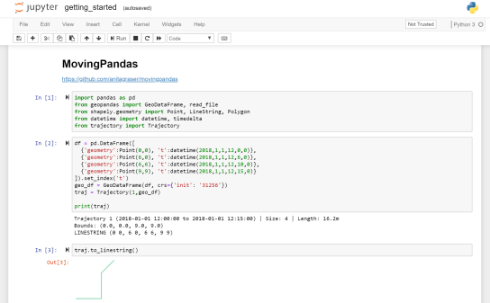
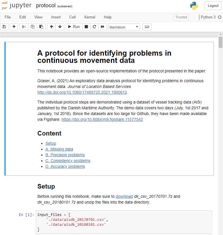
After writing “Towards a template for exploring movement data” last year, I spent a lot of time thinking about how to develop a solid approach for movement data exploration that would help analysts and scientists to better understand their datasets. Finally, my search led me to the excellent paper “A protocol for data exploration to avoid common statistical problems” by Zuur et al. (2010). What they had done for the analysis of common ecological datasets was very close to what I was trying to achieve for movement data. I followed Zuur et al.’s approach of a exploratory data analysis (EDA) protocol and combined it with a typology of movement data quality problems building on Andrienko et al. (2016). Finally, I brought it all together in a Jupyter notebook implementation which you can now find on Github.

There are two options for running the notebook:

1. The repo contains a Dockerfile you can use to spin up a container including all necessary datasets and a fitting Python environment.
2. Alternatively, you can download the datasets manually and set up the Python environment using the provided environment.yml file.

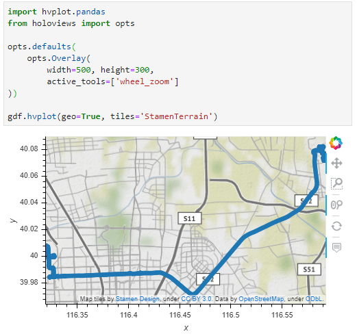
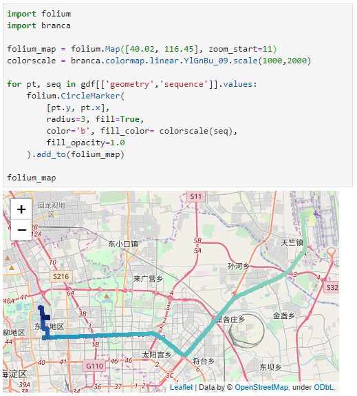
The dataset contains over 10 million location records. Most visualizations are based on Holoviz Datashader with a sprinkling of MovingPandas for visualizing individual trajectories.

Point density map of 10 million location records, visualized using Datashader

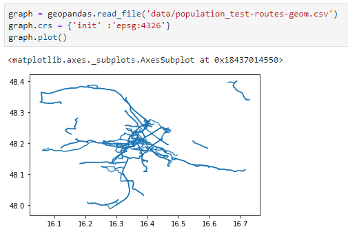
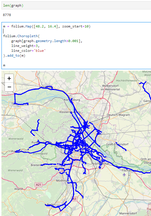
Line density map for detecting gaps in tracks, visualized using Datashader

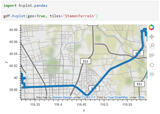
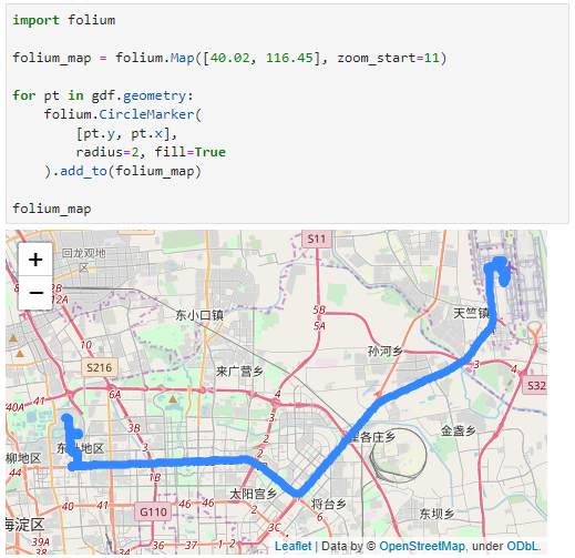
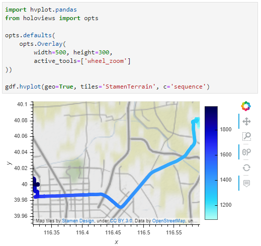
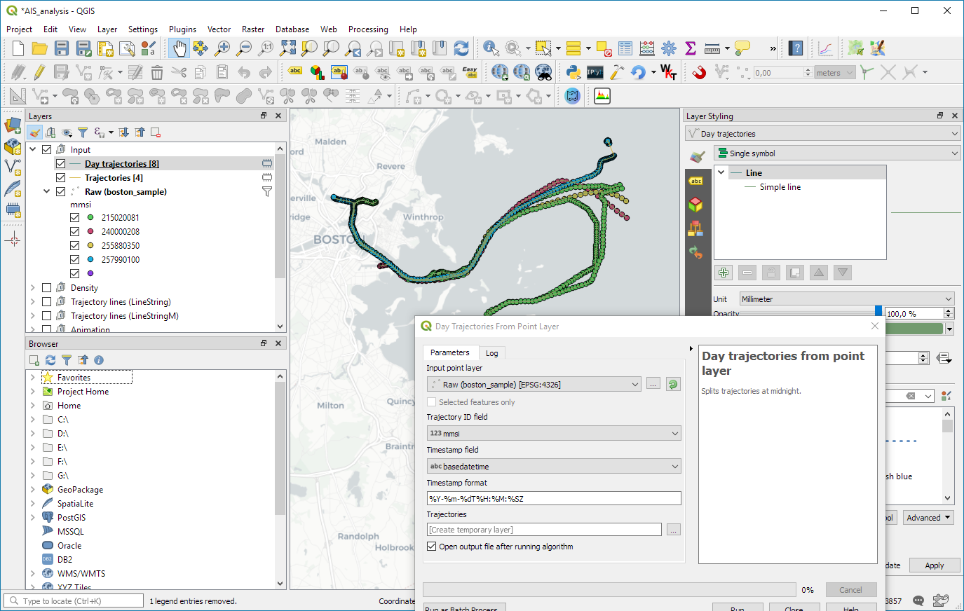
Example trajectory with strong jitter, visualized using MovingPandas & GeoViews

I hope this reference implementation will provide a starting point for many others who are working with movement data and who want to structure their data exploration workflow.

If you want to dive deeper, here’s the paper:

[1] Graser, A. (2021). An exploratory data analysis protocol for identifying problems in continuous movement data. Journal of Location Based Services. doi:10.1080/17489725.2021.1900612.

(If you don’t have institutional access to the journal, the publisher provides 50 free copies using this link. Once those are used up, just leave a comment below and I can email you a copy.)

References

• Zuur, A. F., Ieno, E. N., & Elphick, C. S. (2010). A protocol for data exploration to avoid common statistical problems. Methods in ecology and evolution, 1(1), 3-14. https://doi.org/10.1111/j.2041-210X.2009.00001.x.
• Andrienko, G., Andrienko, N., & Fuchs, G. (2016). Understanding movement data quality. Journal of location Based services, 10(1), 31-46. doi:10.1080/17489725.2016.1169322.

This post is part of a series. Read more about movement data in GIS.

Data sourcing and preparation is one of the most time consuming tasks in many spatial analyses. Even though the Austrian data.gv.at platform already provides a central catalog, the individual datasets still vary considerably in their accessibility or readiness for use.

OGD.AT Lab is a new repository collecting Jupyter notebooks for working with Austrian Open Government Data and other auxiliary open data sources. The notebooks illustrate different use cases, including so far:

1. Accessing geodata from the city of Vienna WFS
2. Downloading environmental data (heat vulnerability and air quality)
3. Geocoding addresses and getting elevation information
4. Exploring urban movement data

Data processing and visualization are performed using Pandas, GeoPandas, and Holoviews. GeoPandas makes it straighforward to use data from WFS. Therefore, OGD.AT Lab can provide one universal gdf_from_wfs() function which takes the desired WFS layer as an argument and returns a GeoPandas.GeoDataFrame that is ready for analysis:

Launch this notebook in: https://mybinder.org/v2/gh/anitagraser/ogd-at-lab/v0.1?urlpath=lab/tree/notebooks/wien-ogd.ipynb

Many other datasets are provided as CSV files which need to be joined with spatial datasets to use them in spatial analysis. For example, the “Urban heat vulnerability index” dataset which needs to be joined to statistical areas.

Launch this notebook in Mybinder: https://mybinder.org/v2/gh/anitagraser/ogd-at-lab/v0.1?urlpath=lab/tree/notebooks/environment.ipynb

Another issue with many CSV files is that they use German number formatting, where commas are used as a decimal separater instead of dots:

Besides file access, there are also open services provided by other developers, for example, Manfred Egger developed an elevation service that provides elevation information for any point in Austria. In combination with geocoding services, such as Nominatim, this makes is possible to, for example, find the elevation for any address in Austria:

Launch this notebook in MyBinder: https://mybinder.org/v2/gh/anitagraser/ogd-at-lab/v0.1?urlpath=lab/tree/notebooks/elevation.ipynb

Last but not least, the first version of the mobility notebook showcases open travel time data provided by Uber Movement:

Launch this notebook in Mybinder: https://mybinder.org/v2/gh/anitagraser/ogd-at-lab/v0.1?urlpath=lab/tree/notebooks/mobility.ipynb

The utility functions for data access included in this repository will continue to grow as new data sources are included. Eventually, it may make sense to extract the data access function into a dedicated library, similar to geofi (Finland) or geobr (Brazil).

If you’re aware of any interesting open datasets or services that should be included in OGD.AT, feel free to reach out here or on Github through the issue tracker or by providing a pull request.

In the previous post, we explored how hvPlot and Datashader can help us to visualize large CSVs with point data in interactive map plots. Of course, the spatial distribution of points usually only shows us one part of the whole picture. Today, we’ll therefore look into how to explore other data attributes by linking other (non-spatial) plots to the map.

This functionality, referred to as “linked brushing” or “crossfiltering” is under active development and the following experiment was prompted by a recent thread on Twitter launched by @plotlygraphs announcement of HoloViews 1.14:

Turns out these features are not limited to plotly but can also be used with Bokeh and hvPlot:

Like in the previous post, this demo uses a Pandas DataFrame with 12 million rows (and HoloViews 1.13.4).

In addition to the map plot, we also create a histogram from the same DataFrame:

map_plot = df.hvplot.scatter(x='x', y='y', datashade=True, height=300, width=400)
hist_plot = df.where((df.SOG>0) & (df.SOG<50)).hvplot.hist("SOG",  bins=20, width=400, height=200) 

To link the two plots, we use HoloViews’ link_selections function:

from holoviews.selection import link_selections
linked_plots = link_selections(map_plot + hist_plot)

That’s all! We can now perform spatial filters in the map and attribute value filters in the histogram and the filters are automatically applied to the linked plots:

Linked brushing demo using ship movement data (AIS): filtering records by speed (SOG) reveals spatial patterns of fast and slow movement.

You’ve probably noticed that there is no background map in the above plot. I had to remove the background map tiles to get rid of an error in Holoviews 1.13.4. This error has been fixed in 1.14.0 but I ran into other issues with the datashaded Scatterplot.

It’s worth noting that not all plot types support linked brushing. For the complete list, please refer to http://holoviews.org/user_guide/Linked_Brushing.html

Even with all their downsides, CSV files are still a common data exchange format – particularly between disciplines with different tech stacks. Indeed, “How to Specify Data Types of CSV Columns for Use in QGIS” (originally written in 2011) is still one of the most popular posts on this blog. QGIS continues to be quite handy for visualizing CSV file contents. However, there are times when it’s just not enough, particularly when the number of rows in the CSV is in the range of multiple million. The following example uses a 12 million point CSV:

To give you an idea of the waiting times in QGIS, I’ve run the following script which loads and renders the CSV:

from datetime import datetime

def get_time():
    t2 = datetime.now()
    print(t2)
    print(t2-t1)
    print('Done :)')

canvas = iface.mapCanvas()
canvas.mapCanvasRefreshed.connect(get_time)

print('Starting ...')

t0 = datetime.now()
print(t0)

print('Loading CSV ...')

uri = "file:///E:/Geodata/AISDK/raw_ais/aisdk_20170701.csv?type=csv&xField=Longitude&yField=Latitude&crs=EPSG:4326&"
vlayer = QgsVectorLayer(uri, "layer name you like", "delimitedtext")

t1 = datetime.now()
print(t1)
print(t1 - t0)

print('Rendering ...')

QgsProject.instance().addMapLayer(vlayer)

The script output shows that creating the vector layer takes 02:39 minutes and rendering it takes over 05:10 minutes:

Starting ...
2020-12-06 12:35:56.266002
Loading CSV ...
2020-12-06 12:38:35.565332
0:02:39.299330
Rendering ...
2020-12-06 12:43:45.637504
0:05:10.072172
Done :)

Rendered CSV file in QGIS

Panning and zooming around are no fun either since rendering takes so long. Changing from a single symbol renderer to, for example, a heatmap renderer does not improve the rendering times. So we need a different solutions when we want to efficiently explore large point CSV files.

The Pandas data analysis library is well-know for being a convenient tool for handling CSVs. However, it’s less clear how to use it as a replacement for desktop GIS for exploring large CSVs with point coordinates. My favorite solution so far uses hvPlot + HoloViews + Datashader to provide interactive Bokeh plots in Jupyter notebooks.

hvPlot provides a high-level plotting API built on HoloViews that provides a general and consistent API for plotting data in (Geo)Pandas, xarray, NetworkX, dask, and others. (Image source: https://hvplot.holoviz.org)

But first things first! Loading the CSV as a Pandas Dataframe takes 10.7 seconds. Pandas’ default plotting function (based on Matplotlib), however, takes around 13 seconds and only produces a static scatter plot.

Loading and plotting the CSV with Pandas

hvPlot to the rescue!

We only need two more steps to get faster and interactive map plots (plus background maps!): First, we need to reproject the lat/lon values. (There’s a warning here, most likely since some of the input lat/lon values are invalid.) Then, we replace plot() with hvplot() and voilà:

Plotting the CSV with Datashader

As you can see from the above GIF, the whole process barely takes 2 seconds and the resulting map plot is interactive and very responsive.

12 million points are far from the limit. As long as the Pandas DataFrame fits into memory, we are good and when the datasets get bigger than that, there are Dask DataFrames. But that’s a story for another day.

The latest v0.5 release is now available from conda-forge.

New features include:

• Stop detection and trajectory splitting at stops
• Improved CRS handling and warnings when CRS is missing

As always, all tutorials are available on MyBinder:

Detected stops (left) and trajectory split at stops (right)

Podcasts have become huge. I’m an avid listener of podcasts myself. I particularly enjoy formats that take the time to talk about unconventional topics in detail.

My first podcast experience was on the QGIS podcast hosted by Tim Sutton in 2014. Unfortunately, it seems like the podcast episodes are not online anymore.

Recently, I had the pleasure to join the MapScaping Podcast by Daniel O’Donohue to talk about Python for Geospatial: 

Other guests Daniel has already interviewed include:

• Kurt Menke talking first about QGIS and in a second episode on QField and Input (data collection apps based on QGIS) and
• Paul Ramsey on Vector Tiles from PostGIS

Another geospatial podcast I really enjoy is The Mappyist Hour by Silas and Todd. Unfortunately, it’s a bit silent there now but it’s definitely worth to listen into their episode archive. One of my favorites is Episode 9 where Linda Stevens (Hecht) discusses her career at ESRI, the future of GIS, and the role of Open Source Spatial in that future:

If you listen to and want to recommend other spatial podcasts, please share them in the comments!

This post introduces Holoviz Panel, a library that makes it possible to create really quick dashboards in notebook environments as well as more sophisticated custom interactive web apps and dashboards.

The following example shows how to use Panel to explore a dataset (a trajectory collection in this case) and different parameter settings (relating to trajectory generalization). All the Panel code we need is a dict that defines the parameters that we want to explore. Then we can use Panel’s interact function to automatically generate a dashboard for our custom plotting function:

import panel as pn

kw = dict(traj_id=(1, len(traj_collection)), 
          tolerance=(10, 100, 10), 
          generalizer=['douglas-peucker', 'min-distance'])
pn.interact(plot_generalized, **kw)

Click to view the resulting dashboard in full resolution:

The plotting function uses the parameters to generate a Holoviews plot. First it fetches a specific trajectory from the trajectory collection. Then it generalizes the trajectory using the specified parameter settings. As you can see, we can easily combine maps and other plots to visualize different aspects of the data:

def plot_generalized(traj_id=1, tolerance=10, generalizer='douglas-peucker'):
  my_traj = traj_collection.get_trajectory(traj_id).to_crs(CRS(4088))
  if generalizer=='douglas-peucker':
    generalized = mpd.DouglasPeuckerGeneralizer(my_traj).generalize(tolerance)
  else:
    generalized = mpd.MinDistanceGeneralizer(my_traj).generalize(tolerance)
  generalized.add_speed(overwrite=True)
  return ( 
    generalized.hvplot(
      title='Trajectory {} (tolerance={})'.format(my_traj.id, tolerance), 
      c='speed', cmap='Viridis', colorbar=True, clim=(0,20), 
      line_width=10, width=500, height=500) + 
    generalized.df['speed'].hvplot.hist(
      title='Speed histogram', width=300, height=500) 
    )

Trajectory collections and generalization functions used in this example are part of the MovingPandas library. If you are interested in movement data analysis, you should check it out! You can find this example notebook in the MovingPandas tutorial section.

In December, I wrote about GeoPandas on Databricks. Back then, I also tried to get MovingPandas working but without luck. (While GeoPandas can be installed using Databricks’ dbutils.library.installPyPI("geopandas") this PyPI install just didn’t want to work for MovingPandas.)

Now that MovingPandas is available from conda-forge, I gave it another try and … *spoiler alert* … it works!

First of all, conda support on Databricks is in beta. It’s not included in the default runtimes. At the time of writing this post, “6.0 Conda Beta” is the latest runtime with conda:

Once the cluster is up and connected to the notebook, a quick conda list shows the installed packages:

Time to install MovingPandas! I went with a 100% conda-forge installation. This takes a looong time (almost half an hour)!

When the installs are finally done, it get’s serious: time to test the imports!

Success!

Now we can put the MovingPandas data structures to good use. But first we need to load some movement data:

Or course, the points in this GeoDataFrame can be plotted. However, the plot isn’t automatically displayed once plot() is called on the GeoDataFrame. Instead, Databricks provides a display() function to display Matplotlib figures:

MovingPandas also uses Matplotlib. Therefore we can use the same approach to plot the TrajectoryCollection that can be created from the GeoDataFrame:

These Matplotlib plots are nice and quick but they lack interactivity and therefore are of limited use for data exploration.

MovingPandas provides interactive plotting (including base maps) using hvplot. hvplot is based on Bokeh and, luckily, the Databricks documentation tells us that bokeh plots can be exported to html and then displayed using  displayHTML():

Of course, we could achieve all this on MyBinder as well (and much more quickly). However, Databricks gets interesting once we can add (Py)Spark and distributed processing to the mix. For example, “Getting started with PySpark & GeoPandas on Databricks” shows a spatial join function that adds polygon information to a point GeoDataFrame.

A potential use case for MovingPandas would be to speed up flow map computations. The recently added aggregator functionality (currently in master only) first computes clusters of significant trajectory points and then aggregates the trajectories into flows between these clusters. Matching trajectory points to the closest cluster could be a potential use case for distributed computing. Each trajectory (or each point) can be handled independently, only the cluster locations have to be broadcast to all workers.

Flow map (screenshot from MovingPandas tutorial 4_generalization_and_aggregation.ipynb)

This post is a follow-up to the draft template for exploring movement data I wrote about in my previous post. Specifically, I want to address step 4: Exploring patterns in trajectory and event data.

The patterns I want to explore in this post are clusters of trip origins. The case study presented here is an extension of the MovingPandas ship data analysis notebook.

The analysis consists of 4 steps:

1. Splitting continuous GPS tracks into individual trips
2. Extracting trip origins (start locations)
3. Clustering trip origins
4. Exploring clusters

Since I have already removed AIS records with a speed over ground (SOG) value of zero from the dataset, we can use the split_by_observation_gap() function to split the continuous observations into individual trips. Trips that are shorter than 100 meters are automatically discarded as irrelevant clutter:

traj_collection.min_length = 100
trips = traj_collection.split_by_observation_gap(timedelta(minutes=5))

The split operation results in 302 individual trips:

Passenger vessel trajectories are blue, high-speed craft green, tankers red, and cargo vessels orange. Other vessel trajectories are gray.

To extract trip origins, we can use the get_start_locations() function. The list of column names defines which columns are carried over from the trajectory’s GeoDataFrame to the origins GeoDataFrame:

 
origins = trips.get_start_locations(['SOG', 'ShipType']) 

The following density-based clustering step is based on a blog post by Geoff Boeing and uses scikit-learn’s DBSCAN implementation:

from sklearn.cluster import DBSCAN
from geopy.distance import great_circle
from shapely.geometry import MultiPoint

origins['lat'] = origins.geometry.y
origins['lon'] = origins.geometry.x
matrix = origins.as_matrix(columns=['lat', 'lon'])

kms_per_radian = 6371.0088
epsilon = 0.1 / kms_per_radian

db = DBSCAN(eps=epsilon, min_samples=1, algorithm='ball_tree', metric='haversine').fit(np.radians(matrix))
cluster_labels = db.labels_
num_clusters = len(set(cluster_labels))
clusters = pd.Series([matrix[cluster_labels == n] for n in range(num_clusters)])
print('Number of clusters: {}'.format(num_clusters))

Resulting in 69 clusters.

Finally, we can add the cluster labels to the origins GeoDataFrame and plot the result:

origins['cluster'] = cluster_labels

To analyze the clusters, we can compute summary statistics of the trip origins assigned to each cluster. For example, we compute a representative (center-most) point, count the number of trips, and compute the mean speed (SOG) value:

 
def get_centermost_point(cluster):
    centroid = (MultiPoint(cluster).centroid.x, MultiPoint(cluster).centroid.y)
    centermost_point = min(cluster, key=lambda point: great_circle(point, centroid).m)
    return Point(tuple(centermost_point)[1], tuple(centermost_point)[0])
centermost_points = clusters.map(get_centermost_point) 

The largest cluster with a low mean speed (indicating a docking or anchoring location) is cluster 29 which contains 43 trips from passenger vessels, high-speed craft, an an undefined vessel:

To explore the overall cluster pattern, we can plot the clusters colored by speed and scaled by the number of trips:

Besides cluster 29, this visualization reveals multiple smaller origin clusters with low speeds that indicate different docking locations in the analysis area.

Cluster locations with high speeds on the other hand indicate locations where vessels enter the analysis area. In a next step, it might be interesting to compute flows between clusters to gain insights about connections and travel times.

It’s worth noting that AIS data contains additional information, such as vessel status, that could be used to extract docking or anchoring locations. However, the workflow presented here is more generally applicable to any movement data tracks that can be split into meaningful trips.

For the full interactive ship data analysis tutorial visit https://mybinder.org/v2/gh/anitagraser/movingpandas/binder-tag

This post is part of a series. Read more about movement data in GIS.

Exploring new datasets can be challenging. Addressing this challenge, there is a whole field called exploratory data analysis that focuses on exploring datasets, often with visual methods.

Concerning movement data in particular, there’s a comprehensive book on the visual analysis of movement by Andrienko et al. (2013) and a host of papers, such as the recent state of the art summary by Andrienko et al. (2017).

However, while the literature does provide concepts, methods, and example applications, these have not yet translated into readily available tools for analysts to use in their daily work. To fill this gap, I’m working on a template for movement data exploration implemented in Python using MovingPandas. The proposed workflow consists of five main steps:

1. Establishing an overview by visualizing raw input data records
2. Putting records in context by exploring information from consecutive movement data records (such as: time between records, speed, and direction)
3. Extracting trajectories & events by dividing the raw continuous tracks into individual trajectories and/or events
4. Exploring patterns in trajectory and event data by looking at groups of the trajectories or events
5. Analyzing outliers by looking at potential outliers and how they may challenge preconceived assumptions about the dataset characteristics

To ensure a reproducible workflow, I’m designing the template as a a Jupyter notebook. It combines spatial and non-spatial plots using the awesome hvPlot library:

This notebook is a work-in-progress and you can follow its development at http://exploration.movingpandas.org. Your feedback is most welcome!

References

• Andrienko G, Andrienko N, Bak P, Keim D, Wrobel S (2013) Visual analytics of movement. Springer Science & Business Media.
• Andrienko G, Andrienko N, Chen W, Maciejewski R, Zhao Y (2017) Visual Analytics of Mobility and Transportation: State of the Art and Further Research Directions. IEEE Transactions on Intelligent Transportation Systems 18(8):2232–2249, DOI 10.1109/TITS.2017.2683539

Over the last years, many data analysis platforms have added spatial support to their portfolio. Just two days ago, Databricks have published an extensive post on spatial analysis. I took their post as a sign that it is time to look into how PySpark and GeoPandas can work together to achieve scalable spatial analysis workflows.

If you sign up for Databricks Community Edition, you get access to a toy cluster for experimenting with (Py)Spark. This considerably lowers the entry barrier to Spark since you don’t need to bother with installing anything yourself. They also provide a notebook environment:

I’ve followed the official Databricks GeoPandas example notebook but expanded it to read from a real geodata format (GeoPackage) rather than from CSV.

I’m using test data from the MovingPandas repository: demodata_geolife.gpkg contains a hand full of trajectories from the Geolife dataset. Demodata_grid.gpkg contains a simple 3×4 grid that covers the same geographic extent as the geolife sample:

Once the files are downloaded, we can use GeoPandas to read the GeoPackages:

Note that the display() function is used to show the plot.

The same applies to the grid data:

When the GeoDataFrames are ready, we can start using them in PySpark. To do so, it is necessary to convert from GeoDataFrame to PySpark DataFrame. Therefore, I’ve implemented a simple function that performs the conversion and turn the Point geometries into lon and lat columns:

To compute new values for our DataFrame, we can use existing or user-defined functions (UDF). Here’s a simple hello world function and associated UDF:

A spatial UDF is a little more involved. For example, here’s an UDF that finds the first polygon that intersects the specified lat/lon and returns that polygon’s ID. Note how we first broadcast the grid DataFrame to ensure that it is available on all computation nodes:

It’s worth noting that PySpark has its peculiarities. Since it’s a Python wrapper of a strongly typed language, we need to pay close attention to types in our Python code. For example, when defining UDFs, if the specified return type (Integertype in the above example) does not match the actual value returned by the find_intersection() function, this will cause rather cryptic errors.

To plot the results, I’m converting the joined PySpark DataFrame back to GeoDataFrame:

I’ve published this notebook so you can give it a try. (Any notebook published on Databricks is supposed to stay online for six months, so if you’re trying to access it after June 2020, this link may be broken.)

In the previous post, I showed how Folium can be used to create interactive maps of GeoPandas GeoDataFrames. Today’s post continues this theme. Specifically, it compares Folium to another dataviz library called hvplot. hvplot also recently added support for GeoDataFrames, so it’s interesting to see how these different solutions compare.

Minimum viable

The following snippets show the minimum code I found to put a GeoDataFrame of Points onto a map with either Folium or hvplot.

Folium does not automatically zoom to the data extent and I didn’t find a way to add the whole GeoDataFrame of Points without looping through the rows individually:

Hvplot on the other hand registers the hvplot function directly with the GeoDataFrame. This makes it as convenient to use as the original GeoPandas plot function. It also zooms to the data extent:

Standard interaction and zoom to area of interest

The following snippets ensure that the map is set to a useful extent and the map tools enable panning and zooming.

With Folium, we have to set the map center and the zoom. The map tools are Leaflet defaults, so panning and zooming work as expected:

Since hvplot does not come with mouse wheel zoom enabled by default, we need to set that:

Color by attribute

Finally, for many maps, we want to show the point location as well as an attribute value.

To create a continuous color ramp for a numeric value, we can use branca.colormap to define the marker fill color:

In hvplot, it is sufficient to specify the attribute of interest:

I’m pretty impressed with hvplot. The integration with GeoPandas is very smooth. Just don’t forget to set the geo=True parameter if you want to plot lat/lon geometries.

Folium seems less straightforward for this use case. Maybe I missed some option similar to the Choropleth function that I showed in the previous post.

GeoPandas makes it easy to create basic visualizations of GeoDataFrames:

However, if we want interactive plots, we need additional libraries. Folium (which is built on Leaflet) is a great option. However, all examples for plotting GeoDataFrames that I found focused on point or polygon data. So here is what I found to work for GeoDataFrames of LineStrings:

First, some imports:

import pandas as pd
import geopandas
import folium

Loading the data:

graph = geopandas.read_file('data/population_test-routes-geom.csv')
graph.crs = {'init' :'epsg:4326'}

Creating the map using folium.Choropleth:

m = folium.Map([48.2, 16.4], zoom_start=10)

folium.Choropleth(
    graph[graph.geometry.length>0.001],
    line_weight=3,
    line_color='blue'
).add_to(m)

m

I also tried using folium.PolyLine which seemed like the more obvious choice but does not seem to accept GeoDataFrames as input. Instead, it expects a list of coordinate pairs and of course it expects them to be in the opposite order that Shapely.LineString.coords provides … Oh the joys of geodata!

In any case, I had to limit the number of features that get plotted because Folium refuses to plot all 8778 features at once. I decided to filter by line length because drawing really short lines is pointless for my overview visualization anyway.

Last week, I had the pleasure to give a movement data analysis workshop at the OpenGeoHub summer school at the University of Münster in Germany. The workshop materials consist of three Jupyter notebooks that have been designed to also support self-study outside of a workshop setting. So you can try them out as well!

All materials are available on Github:

• Tutorial 0 provides an introduction to the MovingPandas Trajectory class.
• Tutorials 1 and 2 provide examples with real-world datasets covering one day of ship movement near Gothenburg and multiple years of gull migration, respectively.

Here’s a quick preview of the bird migration data analysis tutorial (click for full size):

Tutorial 2: Bird migration data analysis

You can run all three Jupyter notebooks online using MyBinder (no installations required).

Alternatively or if you want to dig deeper: installation instructions are available on movingpandas.org

The OpenGeoHub summer school this year had a strong focus on spatial analysis with R and GRASS (sometimes mixing those two together). It was great to meet @mdsumner (author of R trip) and @edzerpebesma (author of R trajectories) for what might have well been the ultimate movement data libraries geek fest. In the ultimate R / Python cross-over, @robinlovelace even ported tutorial 0 to Rmd, so it can be run in RStudio: 0_getting_started.Rmd

Both talks and workshops have been recorded. Here’s the introduction:

and this is the full workshop recording:

This post is part of a series. Read more about movement data in GIS.

Today’s post continues where “Why you should be using PostGIS trajectories” leaves off. It’s the result of a collaboration with Eva Westermeier. I had the pleasure to supervise her internship at AIT last year and also co-supervised her Master’s thesis [0] on the topic of enriching trajectories with information about their geographic context.

Context-aware analysis of movement data is crucial for different domains and applications, from transport to ecology. While there is a wealth of data, efficient and user-friendly contextual trajectory analysis is still hampered by a lack of appropriate conceptual approaches and practical methods. (Westermeier, 2018)

Part of the work was focused on evaluating different approaches to adding context information from vector datasets to trajectories in PostGIS. For example, adding land cover context to animal movement data or adding information on anchoring and harbor areas to vessel movement data.

Classic point-based model vs. line-based model

The obvious approach is to intersect the trajectory points with context data. This is the classic point data model of contextual trajectories. It’s straightforward to add context information in the point-based model but it also generates large numbers of repeating annotations. In contrast, the line data model using, for example, PostGIS trajectories (LinestringM) is more compact since trajectories can be split into segments at context borders. This creates one annotation per segment and the individual segments are convenient to analyze (as described in part #12).

Spatio-temporal interpolation as provided by the line data model offers additional advantages for the analysis of annotated segments. Contextual segments start and end at the intersection of the trajectory linestring with context polygon borders. This means that there are no gaps like in the point-based model. Consequently, while the point-based model systematically underestimates segment length and duration, the line-based approach offers more meaningful segment length and duration measurements.

Schematic illustration of a subset of an annotated trajectory in two context classes, a) systematic underestimation of length or duration in the point data model, b) full length or duration between context polygon borders in the line data model (source: Westermeier (2018))

Another issue of the point data model is that brief context changes may be missed or represented by just one point location. This makes it impossible to compute the length or duration of the respective context segment. (Of course, depending on the application, it can be desirable to ignore brief context changes and make the annotation process robust towards irrelevant changes.)

Schematic illustration of context annotation for brief context changes, a) and b)
two variants for the point data model, c) gapless annotation in the line data model (source: Westermeier (2018) based on Buchin et al. (2014))

Beyond annotations, context can also be considered directly in an analysis, for example, when computing distances between trajectories and contextual point objects. In this case, the point-based approach systematically overestimates the distances.

Schematic illustration of distance measurement from a trajectory to an external
object, a) point data model, b) line data model (source: Westermeier (2018))

The above examples show that there are some good reasons to dump the classic point-based model. However, the line-based model is not without its own issues.

Issues

Computing the context annotations for trajectory segments is tricky. The main issue is that ST_Intersection drops the M values. This effectively destroys our trajectories! There are ways to deal with this issue – and the corresponding SQL queries are published in the thesis (p. 38-40) – but it’s a real bummer. Basically, ST_Intersection only provides geometric output. Therefore, we need to reconstruct the temporal information in order to create usable trajectory segments.

Finally, while the line-based model is well suited to add context from other vector data, it is less useful for context data from continuous rasters but that was beyond the scope of this work.

Conclusion

After the promising results of my initial investigations into PostGIS trajectories, I was optimistic that context annotations would be a straightforward add-on. The line-based approach has multiple advantages when it comes to analyzing contextual segments. Unfortunately, generating these contextual segments is much less convenient and also slower than I had hoped. Originally, I had planned to turn this work into a plugin for the Processing toolbox but the results of this work motivated me to look into other solutions. You’ve already seen some of the outcomes in part #20 “Trajectools v1 released!”.

References

[0] Westermeier, E.M. (2018). Contextual Trajectory Modeling and Analysis. Master Thesis, Interfaculty Department of Geoinformatics, University of Salzburg.

This post is part of a series. Read more about movement data in GIS.

When QGIS 3.0 was release, I published a Processing script template for QGIS3. While the script template is nicely pythonic, it’s also pretty long and daunting for non-programmers. This fact didn’t go unnoticed and Nathan Woodrow in particular started to work on a QGIS enhancement proposal to improve the situation and make writing Processing scripts easier, while – at the same time – keeping in line with common Python styles.

While the previous template had 57 lines of code, the new template only has 26 lines – 50% less code, same functionality! (Actually, this template provides more functionality since it also tracks progress and ensures that the algorithm can be cancelled.)

from qgis.processing import alg
from qgis.core import QgsFeature, QgsFeatureSink

@alg(name="ex_new", label=alg.tr("Example script (new style)"), group="examplescripts", group_label=alg.tr("Example Scripts"))
@alg.input(type=alg.SOURCE, name="INPUT", label="Input layer")
@alg.input(type=alg.SINK, name="OUTPUT", label="Output layer")
def testalg(instance, parameters, context, feedback, inputs):
    """
    Description goes here. (Don't delete this! Removing this comment will cause errors.)
    """
    source = instance.parameterAsSource(parameters, "INPUT", context)

    (sink, dest_id) = instance.parameterAsSink(
        parameters, "OUTPUT", context,
        source.fields(), source.wkbType(), source.sourceCrs())

    total = 100.0 / source.featureCount() if source.featureCount() else 0
    features = source.getFeatures()
    for current, feature in enumerate(features):
        if feedback.isCanceled():
            break
        out_feature = QgsFeature(feature)
        sink.addFeature(out_feature, QgsFeatureSink.FastInsert)
        feedback.setProgress(int(current * total))

    return {"OUTPUT": dest_id}

The key improvement are the new decorators that turn an ordinary function (such as testalg in the template) into a Processing algorithm. Decorators start with @ and are written above a function definition. The @alg decorator declares that the following function is a Processing algorithm, defines its name and assigns it to an algorithm group. The @alg.input decorator creates an input parameter for the algorithm. Similarly, there is a @alg.output decorator for output parameters.

For a longer example script, check out the original QGIS enhancement proposal thread!

For now, this new way of writing Processing scripts is only supported by QGIS 3.6 but there are plans to back-port this improvement to 3.4 once it is more mature. So give it a try and report back!

In previous posts, I already wrote about Trajectools and some of the functionality it provides to QGIS Processing including:

• Creating trajectories from points
• Clipping trajectories by extent
• Splitting trajectories by date

There are also tools to compute heading and speed which I only talked about on Twitter.

Trajectools is now available from the QGIS plugin repository.

The plugin includes sample data from MarineCadastre downloads and the Geolife project.

Under the hood, Trajectools depends on GeoPandas!

If you are on Windows, here’s how to install GeoPandas for OSGeo4W:

1. OSGeo4W installer: install python3-pip
2. Environment variables: add GDAL_VERSION = 2.3.2 (or whichever version your OSGeo4W installation currently includes)
3. OSGeo4W shell: call C:\OSGeo4W64\bin\py3_env.bat
4. OSGeo4W shell: pip3 install geopandas (this will error at fiona)
5. From https://www.lfd.uci.edu/~gohlke/pythonlibs/#fiona: download Fiona-1.7.13-cp37-cp37m-win_amd64.whl
6. OSGeo4W shell: pip3 install path-to-download\Fiona-1.7.13-cp37-cp37m-win_amd64.whl
7. OSGeo4W shell: pip3 install geopandas
8. (optionally) From https://www.lfd.uci.edu/~gohlke/pythonlibs/#rtree: download Rtree-0.8.3-cp37-cp37m-win_amd64.whl and pip3 install it

If you want to use this functionality outside of QGIS, head over to my movingpandas project!

Yesterday, I learned about a cool use case in data-driven agriculture that requires dealing with delayed measurements. As Bert mentions, for example, potatoes end up in the machines and are counted a few seconds after they’re actually taken out of the ground:

Therefore, in order to accurately map yield, we need to take this temporal offset into account.

We need to make sure that time and location stay untouched, but need to shift the potato count value. To support this use case, I’ve implemented apply_offset_seconds() for trajectories in movingpandas:

    def apply_offset_seconds(self, column, offset):
        self.df[column] = self.df[column].shift(offset, freq='1s')

The following test illustrates its use: you can see how the value column is shifted by 120 second. Geometry and time remain unchanged but the value column is shifted accordingly. In this test, we look at the row with index 2 which we access using iloc[2]:

    def test_offset_seconds(self):
        df = pd.DataFrame([
            {'geometry': Point(0, 0), 't': datetime(2018, 1, 1, 12, 0, 0), 'value': 1},
            {'geometry': Point(-6, 10), 't': datetime(2018, 1, 1, 12, 1, 0), 'value': 2},
            {'geometry': Point(6, 6), 't': datetime(2018, 1, 1, 12, 2, 0), 'value': 3},
            {'geometry': Point(6, 12), 't': datetime(2018, 1, 1, 12, 3, 0), 'value':4},
            {'geometry': Point(6, 18), 't': datetime(2018, 1, 1, 12, 4, 0), 'value':5}
        ]).set_index('t')
        geo_df = GeoDataFrame(df, crs={'init': '31256'})
        traj = Trajectory(1, geo_df)
        traj.apply_offset_seconds('value', -120)
        self.assertEqual(traj.df.iloc[2].value, 5)
        self.assertEqual(traj.df.iloc[2].geometry, Point(6, 6))

Pandas is great for data munging and with the help of GeoPandas, these capabilities expand into the spatial realm.

With just two lines, it’s quick and easy to transform a plain headerless CSV file into a GeoDataFrame. (If your CSV is nice and already contains a header, you can skip the header=None and names=FILE_HEADER parameters.)

usecols=USE_COLS is also optional and allows us to specify that we only want to use a subset of the columns available in the CSV.

After the obligatory imports and setting of variables, all we need to do is read the CSV into a regular DataFrame and then construct a GeoDataFrame.

import pandas as pd
from geopandas import GeoDataFrame
from shapely.geometry import Point

FILE_NAME = "/temp/your.csv"
FILE_HEADER = ['a', 'b', 'c', 'd', 'e', 'x', 'y']
USE_COLS = ['a', 'x', 'y']

df = pd.read_csv(
    FILE_NAME, delimiter=";", header=None,
    names=FILE_HEADER, usecols=USE_COLS)
gdf = GeoDataFrame(
    df.drop(['x', 'y'], axis=1),
    crs={'init': 'epsg:4326'},
    geometry=[Point(xy) for xy in zip(df.x, df.y)])

It’s also possible to create the point objects using a lambda function as shown by weiji14 on GIS.SE.

MovingPandas is my attempt to provide a pure Python solution for trajectory data handling in GIS. MovingPandas provides trajectory classes and functions built on top of GeoPandas. 

To lower the entry barrier to getting started with MovingPandas, there’s now an interactive iPython notebook hosted on MyBinder. This notebook provides all the necessary imports and demonstrates how to create a Trajectory object.

Launch MyBinder for MovingPandas to get started!