Today, I’ve been experimenting with data from OpenFlights.org. They offer airport, airline and route data for download. The first idea that came to mind was to connect airports on a shared route by lines. This kind of visualization just looks much nicer if the connections are curved instead of simple straight lines.

Luckily, that’s pretty easy to do using PostGIS. After loading airport positions and route data, we can create the connection lines like this (based on [postgis-users] Great circle as a linestring):

UPDATE experimental.airroutes
SET the_geom =
(SELECT ST_Transform(ST_Segmentize(ST_MakeLine(
       ST_Transform(a.the_geom, 953027),
       ST_Transform(b.the_geom, 953027)
     ), 100000 ), 4326 )
 FROM experimental.airports a, experimental.airports b
 WHERE a.id = airroutes.source_id
   AND b.id = airroutes.dest_id
);

The CRS used in the query is not available in PostGIS by default. You can add it like this (source: spatialreference.org):

INSERT into spatial_ref_sys (srid, auth_name, auth_srid, proj4text, srtext) values ( 953027, 'esri', 53027, '+proj=eqdc +lat_0=0 +lon_0=0 +lat_1=60 +lat_2=60 +x_0=0 +y_0=0 +a=6371000 +b=6371000 +units=m +no_defs ', 'PROJCS["Sphere_Equidistant_Conic",GEOGCS["GCS_Sphere",DATUM["Not_specified_based_on_Authalic_Sphere",SPHEROID["Sphere",6371000,0]],PRIMEM["Greenwich",0],UNIT["Degree",0.017453292519943295]],PROJECTION["Equidistant_Conic"],PARAMETER["False_Easting",0],PARAMETER["False_Northing",0],PARAMETER["Central_Meridian",0],PARAMETER["Standard_Parallel_1",60],PARAMETER["Standard_Parallel_2",60],PARAMETER["Latitude_Of_Origin",0],UNIT["Meter",1],AUTHORITY["EPSG","53027"]]');

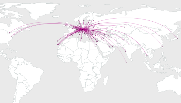
This is an example visualization (done in QGIS) showing only flight routes starting from Vienna International Airport:

Flight routes from Vienna International

Connections crossing the date line are currently more problematic. Lines would have to be split, otherwise this is what you’ll get:

Date line trouble

Want to finally try QGIS Server on your Windows system? Thankfully, Till Adams has written a new HowTo for QGIS Server on Windows. Till shows how to install OSGeo4W version and how to get it running.

If you first want to see what QGIS Server and QGIS Webclient can do, check Webgis-Uster homepage by Andreas Neumann.

Vienna’s Open Government Data initiative is publishing an increasing amount of Geodata and the best thing is: They’re publishing it via open standardized services! Both WMS and WFS are available and ready to be used in QGIS.

Let’s see how we can use the data available through their WFS using the district information layer “Bezirksgrenzen” as an example. The page lists a GML and a GeoJSON version of WFS. For now, we’ll use GeoJSON.

In QGIS, the layer can be loaded using “Add vector layer” – “Protocol” and inserting the GeoJSON url there. The encoding should be changed to ISO8859-15 to account for “Umlaute”.

The loaded GeoJSON layer "Bezirksgrenzen"

Now, we have geodata. Let’s add some attribute data too! Attribute data is available in CSV format. After downloading e.g. some information on the district population, check the file content and remove excessive header lines so that there is only one header line containing attribute names left. Then, you can load the CSV file into QGIS too (“Add vector layer”).

Last step: Joining geodata and attribute data! Go to the vector layer’s properties – Join tab and add the following join relation:

Joining GeoJSON and attribute layer

Now, the attribute table of the vector layer contains the additional CSV attributes – ready for further analysis. If you want to classify based on numerical CSV attributes, you’ll have to create a .csvt file first otherwise all fields are interpreted as texts.

Works great. Thumbs up for this great initiative!

QGIS 1.7 has landed. After some delays due to a major infrastructure overhaul, a new version of QGIS is available for download. For a list of what’s new in 1.7 check the release announcement.

Ever wondered how to create multi-line labels in QGIS? The new labeling engine has a “Multiline labels” option but it’s not so obvious how to create a usable labeling attribute. Here is how it works (credits to @nhopton on QGIS forum):

1. Create a big enough text field (if the data doesn’t contain any yet).
2. In Layer Properties – Fields, chose a “Text edit” edit widget for the label field.
3. Enter the multi-line text into the label field. You can do this using Attribute Table or Feature Form.
   

   A feature form with "Text edit" widget

4. Activate labeling. You’ll have to tick “Multiline labels” option in Layer Labeling Settings – Advanced – Options. That’s it:
   

   Simple multi-line label example

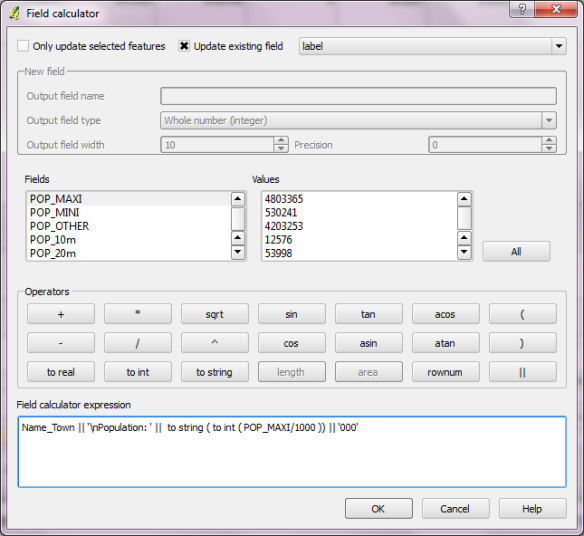
A common use case is the wish to show multiple attribute values in a feature’s label. Using Field Calculator, you can combine them into multi-line labels. All you need is to combine the fields with the || operator and add ‘\n’ (newline) wherever there should be a line break:

Field1 || '\n' || Field2

Populating a multi-line label field using Field Calculator

And finally, the result:

Multi-line labels displaying city name and population

“-T”, this small appendix can be found after many popular GIS-related acronym. But of course, it always means something different. Take for example GIS-T (GIS for Transportation), WFS-T (Transactional WFS) and WMS-T (WMS with time support). The world of acronyms is a fun place!

Let’s see what a WMS-T can do for us. From the WMS standard:

Some geographic information may be available at multiple times (for example, an hourly weather map). A WMS
may announce available times in its service metadata, and the GetMap operation includes a parameter for
requesting a particular time. [...] Depending on the context, time
values may appear as a single value, a list of values, or an interval, …

Currently, only Mapserver supports WMS-T but the Geoserver team is working on it.

Mapserver

MapServer 4.4 and above provides support to interpret the TIME parameter and transform the resulting values into appropriate requests.

Time attributes are specified within the metadata section:

METADATA
"wms_title" "Earthquakes"
"wms_timeextent" "2011-06-01/2011-07-01"
"wms_timeitem" "TIME"
"wms_timedefault" "2011-06-10 12:10:00"
END

Mapserver supports temporal queries for single values, multiple values, single range values or even multiple range values:

...&TIME=2011-06-10&...
...&TIME=2011-06-10, 2004-10-13, 2011-06-19&...
...&TIME=2011-06-10/2011-06-13&...
...&TIME=2011-06-10/2011-06-15, 2011-06-20/2011-06-25&...

Geoserver

GeoSolutions has developed support for TIME and ELEVATION dimensions in WMS.
There are plans to backport this feature to the stable 2.1.x series after the 2.1.1 release.

Configuration of time-enabled layers can be done via the normal user interface:

The following video by GeoSolutions demonstrates the use of Geoserver’s WMS-T:

Both server solutions seem to support only one time attribute per layer. An optional second time attribute would be nice to support datasets with start and end time like Time Manager for QGIS does.

The gis.stackexchange community keeps on growing and it’s questions and answers span a wide spectrum of GIS-related topics. As of today, the page lists 2,700 questions and 6,400 answers.

As was to be expected, ‘arcgis’ (549 times) is the most used tag followed by ‘arcgis-10.0′ ;)

From an open source perspective, PostGIS gets most attention (rank 8), followed closely by OpenLayers (rank 9) and Geoserver (rank 10). QGIS is the highest-ranked desktop GIS (rank 13). Users of other open source desktop GIS like uDig or gvSIG don’t seem to be using this platform yet.

Here’s the full list of open source GIS tags with a count of more than 10:

postgis × 149
openlayers × 137
geoserver × 121
qgis × 97
open-source × 94
grass × 85
gdal × 68
postgresql × 32
pgrouting × 20
geodjango × 14
mapnik × 13

Recently, @simo has posted an elegant solution for defining custom styles for Google Maps layers in OpenLayers on gis.stackexchange. An example with source can be found at http://www.empreinte-urbaine.eu/mapping/styled_gmap.html. The idea seems to be to use a StyledMapType:

The StyledMapType allows you to customize the presentation of the standard Google base maps, changing the visual display of such elements as roads, parks, and built-up areas to reflect a different style than that used in the default map type.

How great would it be if it was possible to define such styles in QGIS OpenLayers plugin too!

The aim of QGIS Processing Framework developed by Polymeris is to provide a generic framework for accessing existing geo-processing functionality of e.g. SAGA, GRASS, Orfeo Toolbox, etc. This should enable users to script their geo-processing work in python console and allow development of a tool to graphically build workflows using VisTrails an “open-source scientific workflow and provenance management system”.

For a first impression, Polymeris has published some screenshots of QGIS with SAGA modules loaded: [1],[2]

This project is big and if it turns out well, QGIS will profit enormously from it. Both scriptable geoprocessing functionality and a graphic workflow builder can improve user experience a lot if they are implemented well. You can follow further development on the project homepage on GitHub.

On Wednesday, Allan Maungu – geoscripting.blogspot.com announced MXD2QGS, a converter that exports layers from an Arcmap 10 document into a Quantum GIS project file. The tool is built as an ArcToolbox and can be downloaded from the blog.

I’d be very interested to hear whether this tool works for you.

For everyone working with spatial databases in QGIS there comes a time when “Add PostGIS/SpatiaLite Layer” and “RT Sql Layer” start to be annoying. You always have to retype or copy-paste your SQL queries into the user interface if you need to change the tiniest thing in the layer’s definition.

This is where “Fast SQL Layer” can be a real time saver. Fast SQL Layer is a new plugin for QGIS by Pablo T. Carreira. It basically adds an SQL console for loading layers from PostGIS/SpatiaLite into QGIS. And it even comes with syntax highlighting!

Installation

Fast SQL Layer comes with one dependency: Pygments, which is used for syntax highlighting.

On Ubuntu, all you have to do is install it with apt-get:

sudo apt-get install python-pygments

For Windows with OSGeo4W, @Mike_Toews posted this on gis.stackexchange:

I downloaded and extracted Pygments-1.4.tar.gz, then in an OSGeo4W shell within the Pygments-1.4 directory, type python setup.py build then python setup.py install

Usage

When you activate the plugin in plugin manager, a dock widget will appear which contains the console and some fields for specifying the database connection that should be used. Then, you can simply write your SQL query and load the results with one click.

Fast SQL plugin

In this example, I renamed “gid” to “id”, but you can actually edit the values in the drop down boxes to adjust the column names for id and geometry:

A second layer loaded using Fast SQL plugin

It certainly needs some polishing on the user interface side but I really like it.

The city of Vienna has started their open data initiative. They’re offering data on a variety of topics, including: infrastructure, population, education, environment and traffic.

For use in GIS, they serve the data through WMS and WFS:

• WMS: http://data.wien.gv.at/daten/wms?service=WMS&request=GetCapabilities&version=1.1.1
• WFS 1.0: http://data.wien.gv.at/daten/wfs?service=WFS&request=GetCapabilities&version=1.0.0
•  WFS 1.1: http://data.wien.gv.at/daten/wfs?service=WFS&request=GetCapabilities&version=1.1.0

Both WMS and WFS work well with the developer version of QGIS.

Looking forward to new datasets. Announcements should be published via RSS feed.

In a previous post, I’ve described how to create catchment areas with pgRouting shortest_path() function. The solution described there calculates costs from the starting node (aka vertex) to all other nodes in the network. Depending on the network size, this can take a long time. Especially, if you are only interested in relatively small catchment areas (e.g. 50 km around a node in a network covering 10,000 km) there is a lot of unnecessary calculation going on. This is where you might want to use driving_distance() instead.

Driving_distance() offers a parameter for maximum distance/cost and will stop calculations when the costs exceed this limit. But let’s start at the beginning: installing the necessary functions.

Installation

If you have followed my guide to installing pgRouting, you already have some routing functions installed – but not driving_distance(). Weirdly, the necessary SQL scripts are not shipped with the .zip file available on pgRouting’s download page. You need:

routing_dd.sql
routing_dd_wrappers.sql

Both are available through the project repository at Github. Get them and execute them in your pgRouting-enabled database. Now, you should be ready.

Calculating driving distances

To calculate driving distances, we need a query very similar to shortest_path():

CREATE OR REPLACE FUNCTION driving_distance(
sql text,
source_id integer,
distance float8,
directed boolean,
has_reverse_cost boolean)
RETURNS SETOF path_result

The only new value is “distance”. That’s the maximum distance/cost you want to be contained in the result set. “distance” has to be specified in the same units as the cost attribute (which is specified in the “sql” text parameter).

Note: In my opinion, the name “(driving) distance” is misleading. While you can use distance as a cost attribute, you’re not limited to distances. You can use any cost attribute you like, e.g. travel time, fuel consumption, co2 emissions, …

The actual query for a catchment area of 100 km around node # 2000 looks like this:

SELECT * FROM driving_distance('
      SELECT gid AS id,
          start_id::int4 AS source,
          end_id::int4 AS target,
          shape_leng::float8 AS cost
      FROM network',
      2000,
      100000,
      false,
      false)

Interpreting the result

These are the first lines of the result set:

vertex_id;edge_id;cost
294;7262;97400.433506144
297;7236;98012.620979231
335;1095;96849.456306244
347;7263;93617.693852324
364;7098;93573.849081386
366;2551;92702.443434779
378;7263;91994.328368081

The cost attribute contains the total cost of travel from the starting node to the vertex_id node.
We will only be using vertex_id and cost. The use of edge_id is a mystery to me.

Visualizing the result

The easiest way to visualize driving_distance() results is using RT Sql Layer plugin. We need to join the results of driving_distance() with the table containing node geometries:

SELECT *
   FROM node
   JOIN
   (SELECT * FROM driving_distance('
      SELECT gid AS id,
          start_id::int4 AS source,
          end_id::int4 AS target,
          shape_leng::float8 AS cost
      FROM network',
      2000,
      100000,
      false,
      false)) AS route
   ON
   node.id = route.vertex_id

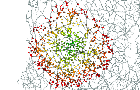
If you color the nodes based on the cost attribute, it will look something like this:

result of pgRouting driving_distance() visualized in QGIS

FOSSGIS2011 in Heidelberg was a great success for the QGIS project and for me personally. The audience was really impressed by Marco’s and Andreas’ presentation on QGIS Mapserver and GeoExt Web Client. My presentation on Time Manager for QGIS was followed by a series of interesting questions and comments concerning use cases in e.g. land use mapping. Requested features include support for raster layers and support for timestamps before year 19xx.
I’ll be posting an English version of the Time Manager presentation including some additional comments here soon.

A great new initiative has been started on QGIS wiki: “How to do X in QGIS” aims at providing step-by-step tutorials for various tasks based on the latest versions of QGIS. This new knowledge base is meant to complement the existing documentation and to replace some of the outdated tutorials available all over the web.

Feel free to contribute tutorials or tutorial ideas, it’s a wiki!

There are many nice examples out there of how to use a getFeatureInfo request in OpenLayers to display a feature’s attribute table. In some applications it can be useful though not to display the full attribute table but to only select one attribute value from it and output it somewhere, e.g. in a text field.

This post describes how to pick the road id from a road wms layer and write the id value into a text input field.

OpenLayers offers a convenient class to achieve this: OpenLayers.Control.WMSGetFeatureInfo.

Let’s create an object of this class, register and activate it:

roadidPicker = new OpenLayers.Control.WMSGetFeatureInfo({
                url: 'http://localhost:8080/geoserver/wms',
                title: 'identify features on click',
                layers: [wms],
                queryVisible: true
            });
roadidPicker.infoFormat = 'application/vnd.ogc.gml';
roadidPicker.events.register("getfeatureinfo", this, pickRoadid);
map.addControl(roadidPicker);
roadidPicker.activate();

Now, every time the user clicks onto the map, a getFeatureInfo request is issued and the function pickRoadid() is called. In pickRoadid(), we’ll define which value we want to pick from the feature. The ‘id’ of the feature will be written into a text input field called ‘roadId’:

function pickRoadid(e) {
  if (e.features && e.features.length) {
     var val = e.features[0].attributes.id;
     document.getElementById('roadId').value = val;
  }
}

You might have noticed the ‘[0]‘. That’s because the click event comes with a list of features within the reach of the mouse click. For my application, I can only use one value and the first feature in this list is as good as any.

The aim of this post is to describe a method for labeling of a subset of features within a layer using new labeling functionality.

The problem

Often, we want to label only a few features in a layer. Of course we can export those features to a new layer and label them that way, but that requires creation of additional files and layers within your project. Things will start to get messy fast.

Another approach is to delete unwanted label texts from the attribute table. This either means that you have to duplicate a “name” attribute and then start deleting from the newly created attribute table column or that you actually delete values in the original column. Both approaches are problematic. Either you produce redundancy that gets difficult to maintain (two attributes have to be updated if the name of a feature changes) or you loose information from the attribute table.

The suggested solution

Let me present a different approach using new labeling tools. The idea is based on moving unwanted labels out of view. This approach avoids duplication of features and duplication/deletion of label texts. And this is the workflow:

1. Select the features you want to label
2. Open attribute table
3. If you don’t have label attributes ready yet: Add two type “real” columns called e.g. “label_x” and “label_y”
4. Invert the selection (3rd button in attribute table window)
5. Open field calculator and fill “label_x” and “label_y” fields of the selected features with 0 values (or any coordinates outside your map extent)
6. Close field calculator and attribute table
7. Save your edits
8. Open the labeling dialog and set “data defined settings” – “x coordinate” and “y coordinate”
9. Enable “Label this layer” and specify the label field
10. Done

If you change your mind about a feature and want to label it later on: Simply delete the values in “label_x” and “label_y” fields (so they read NULL).

This works quite well for me but I’m aware that it’s still not optimal. Another “data defined setting” like “show this label (true/false)” would be more intuitive.

Have you found better solutions to this problem? Please, post them!

If you load .csv files through “Add vector layer”, all columns are interpreted as strings. That’s most likely not what you want, but it’s OGR’s default behaviour:

The OGR CSV driver returns all attribute columns with a type of string if no field type information file (with .csvt extension) is available.

Let’s create a .csvt file then!

The .csvt file has to have the same name as the .csv file it describes. (Same concept used in shapefiles.) It enables definition of the following data types: Integer, Real, String, Date (YYYY-MM-DD), Time (HH:MM:SS+nn) and DateTime (YYYY-MM-DD HH:MM:SS+nn).

A .csvt file contains only one line and the types for each column have to be quoted and comma separated, e.g.

"Integer","Real","String"

You can even specify width and precision of each column, e.g.

"Integer(6)","Real(5.5)","String(22)"

Read more at: www.gdal.org/ogr/drv_csv.html

CAD Tools is a powerful plugin for QGIS that is intended to improve your digitizing workflow. While it has a lot to offer, the tools are not very self-explanatory – especially for people who are not used to the CAD way of doing things.

Luckily, there is a great learning resource out there. Stefan Ziegler explains the tools and shows their use in a series of screen casts that are easy to follow and reproduce. Enjoy!

We are pleased to announce the release of Time Manager version 0.3. New features include:

• Saving – Time Manager settings are now being saved to the project file.
• Image series export – animations can be exported as image series.
• Help files – The plugin now comes with a user guide / help file.
• Looping animations – When “looping” is enabled, the animation will start over from the beginning instead of stopping when it reaches the end.

Time Manager user guide

Time Manager is available through Geofrogger Repository. Give it a try!