In the past, network analysis capabilities in QGIS were rather limited or not straight-forward to use. This has changed! In QGIS 3.x, we now have a wide range of network analysis tools, both for use case where you want to use your own network data, as well as use cases where you don’t have access to appropriate data or just prefer to use an existing service.

This blog post aims to provide an overview of the options:

1. Based on local network data
   1. Default QGIS Processing network analysis tools
   2. QNEAT3 plugin
2. Based on web services
   1. Hqgis plugin (HERE)
   2. ORS Tools plugin (openrouteservice.org)
   3. TravelTime platform plugin (TravelTime platform)

All five options provide Processing toolbox integration but not at the same level.

If you are a regular reader of this blog, you’re probably also aware of the pgRoutingLayer plugin. However, I’m not including it in this list due to its dependency on PostGIS and its pgRouting extension.

Processing network analysis tools

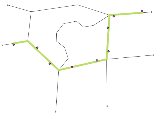
The default Processing network analysis tools are provided out of the box. They provide functionality to compute least cost paths and service areas (distance or time) based on your own network data. Inputs can be individual points or layers of points:

The service area tools return reachable edges and / or nodes rather than a service area polygon:

QNEAT3 plugin

The QNEAT3 (short for Qgis Network Analysis Toolbox 3) Plugin aims to provide sophisticated QGIS Processing-Toolbox algorithms in the field of network analysis. QNEAT3 is integrated in the QGIS3 Processing Framework. It offers algorithms that range from simple shortest path solving to more complex tasks like Iso-Area (aka service areas, accessibility polygons) and OD-Matrix (Origin-Destination-Matrix) computation.

QNEAT3 is an alternative for use case where you want to use your own network data.

For more details see the QNEAT3 documentation at: https://root676.github.io/index.html

Hqgis plugin

Access the HERE API from inside QGIS using your own HERE-API key. Currently supports Geocoding, Routing, POI-search and isochrone analysis.

Hqgis currently does not expose all its functionality to the Processing toolbox:

Instead, the full set of functionality is provided through the plugin GUI:

This plugin requires a HERE API key.

ORS Tools plugin

ORS Tools provides access to most of the functions of openrouteservice.org, based on OpenStreetMap. The tool set includes routing, isochrones and matrix calculations, either interactive in the map canvas or from point files within the processing framework. Extensive attributes are set for output files, incl. duration, length and start/end locations.

ORS Tools is based on OSM data. However, using this plugin still requires an openrouteservice.org API key.

TravelTime platform plugin

This plugin adds a toolbar and processing algorithms allowing to query the TravelTime platform API directly from QGIS. The TravelTime platform API allows to obtain polygons based on actual travel time using several transport modes rather, allowing for much more accurate results than simple distance calculations.

The TravelTime platform plugin requires a TravelTime platform API key.

For more details see: https://blog.traveltimeplatform.com/isochrone-qgis-plugin-traveltime

Wrong navigation instructions can be annoying and sometimes even dangerous, but they happen. No dataset is free of errors. That’s why it’s important to assess the quality of datasets. One specific use case I previously presented at FOSS4G 2013 is the quality assessment of turn restrictions in OSM, which influence vehicle routing results.

The main idea is to compare OSM to another data source. For this example, I used turn restriction data from the City of Toronto. Of the more than 70,000 features in this dataset, I extracted a sample of about 500 turn restrictions around Ryerson University, which I had the pleasure of visiting in 2014.

As you can see from the following screenshot, OSM and the city’s dataset agree on 420 of 504 restrictions (83%), while 36 cases (7%) are in clear disagreement. The remaining cases require further visual inspection.

The following two examples show one case where the turn restriction is modelled in both datasets (on the left) and one case where OSM does not agree with the city data (on the right).
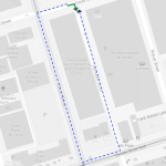
In the first case, the turn restriction (short green arrow) tells us that cars are not allowed to turn right at this location. An OSM-based router (here I used OpenRouteService.org) therefore finds a route (blue dashed arrow) which avoids the forbidden turn. In the second case, the router does not avoid the forbidden turn. We have to conclude that one of the two datasets is wrong.

If you want to learn more about the methodology, please check Graser, A., Straub, M., & Dragaschnig, M. (2014). Towards an open source analysis toolbox for street network comparison: indicators, tools and results of a comparison of OSM and the official Austrian reference graph. Transactions in GIS, 18(4), 510-526. doi:10.1111/tgis.12061.

Interestingly, the disagreement in the second example has been fixed by a recent edit (only 14 hours ago). We can see this in the OSM way history, which reveals that the line direction has been switched, but this change hasn’t made it into the routing databases yet:

This leads to the funny situation that the oneway is correctly displayed on the map but seemingly ignored by the routers:

To evaluate the results of the automatic analysis, I wrote a QGIS script, which allows me to step through the results and visually compare turn restrictions and routing results. It provides a function called next() which updates a project variable called myvar. This project variable controls which features (i.e. turn restriction and associated route) are rendered. Finally, the script zooms to the route feature:

def next():
    f = features.next()
    id = f['TURN_ID']
    print "Going to %s" % (id)
    QgsExpressionContextUtils.setProjectVariable('myvar',id)
    iface.mapCanvas().zoomToFeatureExtent(f.geometry().boundingBox())
    if iface.mapCanvas().scale() < 500:
        iface.mapCanvas().zoomScale(500)

layer = iface.activeLayer()
features = layer.getFeatures()
next()

You can see it in action here:

I’d love to see this as an interactive web map where users can have a look at all results, compare with other routing services – or ideally the real world – and finally fix OSM where necessary.

This work has been in the making for a while. I’d like to thank the team of OpenRouteService.org who’s routing service I used (and who recently added support for North America) as well as my colleagues at Ryerson University in Toronto, who pointed me towards Toronto’s open data.

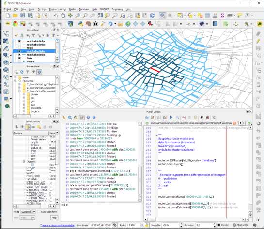
As announced in Salzburg a few days ago, I’m happy to present the lastest enhancement to my IDF router for QGIS: travel time routing and catchment computation.

Travel times for pedestrians and cyclists are computed using constant average speeds, while car travel times depend on the speed values provided by the road network data.

Catchment computations return the links that can be traversed completely within the given time (or distance limit). The current implementation does not deal with links at the edge of the catchment area, which can only be traversed partially.

Loading the whole network (2.7GB unzipped IDF) currently requires around 10GB of memory. One of the next plans therefore is to add a way to only load features within a specified bounding box.

Plans to turn this into a full-blown plugin will most likely have to wait for QGIS 3, which will ship with Python 3 and other updated libraries.

Monday, January 4th 2016, was the open data release date of the official Austrian street network dataset called GIP.at. As far as I know, the dataset is not totally complete yet but it should be in the upcoming months. I’ve blogged about GIP.at before in Open source IDF parser for QGIS and Open source IDF router for QGIS where I was implementing tools based on the data samples that were available then. Naturally, I was very curious if my parser and particularly the router could handle the whole country release …

Some code tweaking, patience for loading, and 9GB of RAM later, QGIS happily routes through Austria, for example from my work place to Salzburg – maybe for some skiing:

The routing request itself takes something between 1 and 2 seconds. (I should still add a timer to it.)

So far, I’ve implemented shortest distance routing for pedestrians, bikes, and cars. Since the data also contains travel speeds, it should be quite straight-forward to also add shortest travel time routing.

The code is available on Github for you to try. I’d appreciate any feedback!

This is a follow-up on my previous post introducing an Open source IDF parser for QGIS. Today’s post takes the code further and adds routing functionality for foot, bike, and car routes including oneway streets and turn restrictions.

You can find the script in my QGIS-resources repository on Github. It creates an IDFRouter object based on an IDF file which you can use to compute routes.

The following screenshot shows an example car route in Vienna which gets quite complex due to driving restrictions. The dark blue line is computed by my script on GIP data while the light blue line is the route from OpenRouteService.org (via the OSM route plugin) on OSM data. Minor route geometry differences are due to slight differences in the network link geometries.

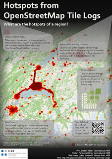
It’s my pleasure to report back from this year’s AGIT and GI_Forum conference (German and English speaking respectively). It was great to meet the gathered GIS crowd! If you missed it, don’t despair: I’ve compiled a personal summary on Storify, and papers (German, English) and posters are available online. Here’s a pick of my favorite posters:

I also had the pleasure to be involved in multiple presentations this year:

QGIS at the OSGeo Day

As part of the OSGeo Day, I had the chance to present the latest and greatest QGIS features for map design in front of a full house:

A. Graser: Kartendesign mit QGis (Top 10 Neuerungen) volles Haus, 2016 im Audimax? #AGIT2015 http://t.co/ShjAOQObg2

—
Jochen Schwarze (@jochens100570) July 10, 2015

Routing with OSM

On a slightly different note, my colleague Markus Straub and I presented an introduction to routing with OpenStreetMap covering which kind of routing-related information is available in OSM as well as a selection of different tools to perform routing on OSM.

Solving the “unnamed link” problem

In this talk, I presented approaches to solving issues with route descriptions that contain unnamed pedestrian or cycle paths.

fight "unknown road" driving directions for #cycling and #pedestrian navigation. @underdarkGIS at #GIForum2015 http://t.co/eRvY51gDsP

—
gicycle (@gicycle_) July 09, 2015

Here you can find the full open access paper: Graser, A., & Straub, M. (2015). Improving Navigation: Automated Name Extraction for Separately Mapped Pedestrian and Cycle Links. GI_Forum ‒ Journal for Geographic Information Science, 1-2015, 546-556, doi:10.1553/giscience2015s546.

Inferring road popularity from GPS trajectories

In this talk, my colleague Markus Straub presented our new approach to computing how popular a certain road is. The resulting popularity value can be used for planning as well as routing.

Popularity as a viable option for computing alternative routes #GIForum2015 http://t.co/SLZFhLyfVa

—
Anita Graser (@underdarkGIS) July 08, 2015

Here you can find the full open access paper: Straub, M., & Graser, A. (2015). Learning from Experts: Inferring Road Popularity from GPS Trajectories. GI_Forum ‒ Journal for Geographic Information Science, 1-2015, 41-50, doi:10.1553/giscience2015s41.

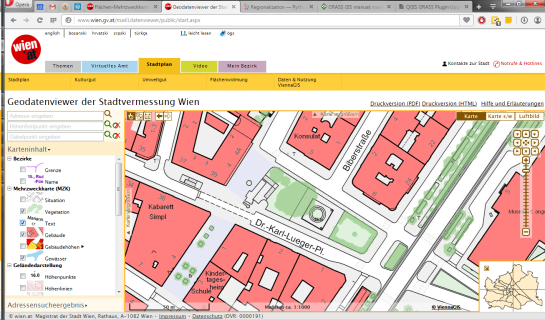
A few weeks ago, the city of Vienna released a great dataset: the so-called “Flächen-Mehrzweckkarte” (FMZK) is a polygon vector layer with an amazing level of detail which contains roads, buildings, sidewalk, parking lots and much more detail:

preview of the Flächen-Mehrzweckkarte

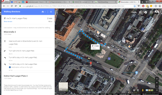
Now, of course we can use this dataset to create gorgeous maps but wouldn’t it be great to use it for analysis? One thing that has been bugging me for a while is routing for pedestrians and how it’s still pretty bad in many situations. For example, if I’d be looking for a route from the northern to the southern side of the square in the previous screenshot, the suggestions would look something like this:

Pedestrian routing in Google Maps

… Great! Google wants me to walk around it …

Pedestrian routing on openstreetmap.org

… Openstreetmap too – but on the other side :P

Wouldn’t it be nice if we could just cross the square? There’s no reason not to. The routing graphs of OSM and Google just don’t contain a connection. Polygon datasets like the FMZK could be a solution to the issue of routing pedestrians over squares. Here’s my first attempt using GRASS r.walk:

Routing with GRASS r.walk (Green areas are walk-friendly, yellow/orange areas are harder to cross, and red buildings are basically impassable.)

… The route crosses the square – like any sane pedestrian would.

The key steps are:

1. Assigning pedestrian costs to different polygon classes
2. Rasterizing the polygons
3. Computing a cost raster for moving using r.walk
4. Computing the route using r.drain

I’ve been using GRASS 7 for this example. GRASS 7 is not yet compatible with QGIS but it would certainly be great to have access to this functionality from within QGIS. You can help make this happen by supporting the crowdfunding initiative for the GRASS plugin update.

Correct turn restriction information is essential for the vehicle routing quality of any street network dataset – open or commercial. One of the challenges of this kind of information is that these restrictions are typically not directly visible on each map.

This post is inspired by a share on G+ which resurfaced in my notifications. In a post on the Mapbox blog, John Firebaugh presents the OSM iD editor which should make editing turn restrictions straight-forward: clicking on the source link turns the associated turn information visible. By clicking on the turn arrows, the user can easily toggle between allowed and forbidden.

editing turn restrictions in iD, the web editor for OpenStreetMap. source: “Simple Editing for Turn Restrictions in OpenStreetMap” by John Firebaugh on June 06 2014

But the issue of identifying wrong turn restrictions remains. One approach to solving this issue is to compare restriction information in OSM with the information in a reference data set.

This is possible by comparing routes computed on OSM and the reference data using a method I presented at FOSS4G (video): a turn restriction basically is a forbidden combination of links. If we compute the route from the start link of the forbidden combination to the end link, we can check if the resulting route geometry violates the restriction or uses an appropriate detour:

illustrative slide from my LBS2014 presentation on OSM vehicle routing quality – read more about this method and results for Vienna in our TGIS paper or the open pre-print version

It would be great to have an automated system comparing OSM and open government street network data to detect these differences. The quality of both data sets could benefit enormously by bundling their QA efforts. Unfortunately, the open government street network data sets I’m aware of don’t contain turn information.

Did you know that there is a network analysis library in QGIS core? It’s well hidden so far, but at least it’s documented in the PyQGIS Cookbook. The code samples from the cookbook can be used in the QGIS Python console and you can play around to get a grip of what the different steps are doing.

As a first exercise, I’ve decided to write a Processing script which will use the network analysis library to create a network-based route layer from a point layer input. You can find the result on Github.

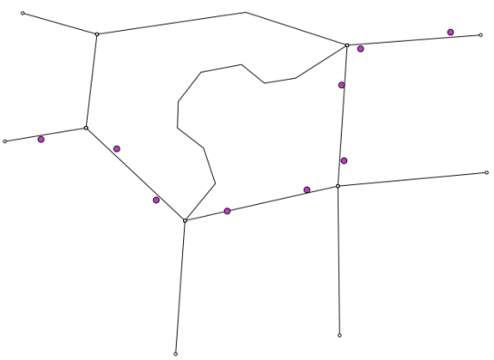
You can get a Spatialite file with testdata from Github as well. It contains a network and a routepoints1 layer:

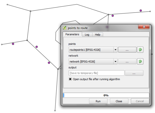
The interface of the points_to_route tool is very simple. All it needs as an input is information about which layer should be used as a network and which layer contains the route points:

The input points are considered to be ordered. The tool always routes between consecutive points.

The result is a line layer with one line feature for each point pair:

The network analysis library is a really great new feature and I hope we will see a lot of tools built on top of it.

This post covers a simple approach to calculating isochrones in a public transport network using pgRouting and QGIS.

For this example, I’m using the public transport network of Vienna which is loaded into a pgRouting-enable database as network.publictransport. To create the routable network run:

select pgr_createTopology('network.publictransport', 0.0005, 'geom', 'id');

Note that the tolerance parameter 0.0005 (units are degrees) controls how far link start and end points can be apart and still be considered as the same topological network node.

To create a view with the network nodes run:

create or replace view network.publictransport_nodes as
select id, st_centroid(st_collect(pt)) as geom
from (
	(select source as id, st_startpoint(geom) as pt
	from network.publictransport
	) 
union
	(select target as id, st_endpoint(geom) as pt
	from network.publictransport
	) 
) as foo
group by id;

To calculate isochrones, we need a cost attribute for our network links. To calculate travel times for each link, I used speed averages: 15 km/h for buses and trams and 32km/h for metro lines (similar to data published by the city of Vienna).

alter table network.publictransport add column length_m integer;
update network.publictransport set length_m = st_length(st_transform(geom,31287));

alter table network.publictransport add column traveltime_min double precision;
update network.publictransport set traveltime_min = length_m  / 15000.0 * 60; -- average is 15 km/h
update network.publictransport set traveltime_min = length_m  / 32000.0 * 60 where "LTYP" = '4'; -- average metro is 32 km/h

That’s all the preparations we need. Next, we can already calculate our isochrone data using pgr_drivingdistance, e.g. for network node #1:

create or replace view network.temp as
 SELECT seq, id1 AS node, id2 AS edge, cost, geom
  FROM pgr_drivingdistance(
    'SELECT id, source, target, traveltime_min as cost FROM network.publictransport',
    1, 100000, false, false
  ) as di
  JOIN network.publictransport_nodes pt
  ON di.id1 = pt.id;

The resulting view contains all network nodes which are reachable within 100,000 cost units (which are minutes in our case).

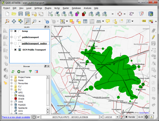
Let’s load the view into QGIS to visualize the isochrones:

The trick is to use data-defined size to calculate the different walking circles around the public transport stops. For example, we can set up 10 minute isochrones which take into account how much time was used to travel by pubic transport and show how far we can get by walking in the time that is left:

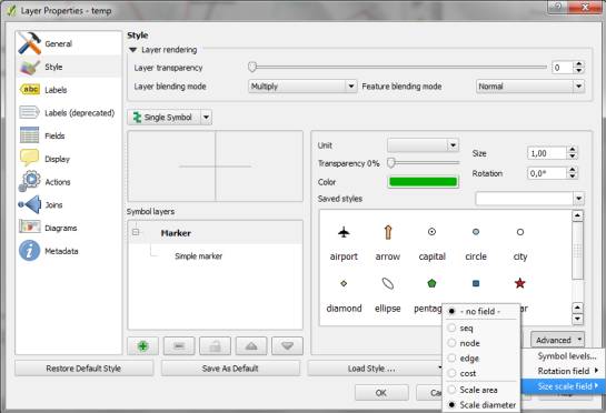
1. We want to scale the circle radius to reflect the remaining time left to walk. Therefore, enable Scale diameter in Advanced | Size scale field:

2. In the Simple marker properties change size units to Map units.
3. Go to data defined properties to set up the dynamic circle size.

The expression makes sure that only nodes reachable within 10 minutes are displayed. Then it calculates the remaining time (10-"cost") and assumes that we can walk 100 meters per minute which is left. It additionally multiplies by 2 since we are scaling the diameter instead of the radius.

To calculate isochrones for different start nodes, we simply update the definition of the view network.temp.

While this approach certainly has it’s limitations, it’s a good place to start learning how to create isochrones. A better solution should take into account that it takes time to change between different lines. While preparing the network, more care should to be taken to ensure that possible exchange nodes are modeled correctly. Some network links might only be usable in one direction. Not to mention that there are time tables which could be accounted for ;)

The function with the glorious name “find_node_by_nearest_link_within_distance” is part of pgRouting and can be found in matching.sql.

“This function finds nearest node as a source or target of the nearest link”
That means that we can use this function e.g. to find the best road network node for a given address.

The function returns an object of type link_point:

CREATE TYPE link_point AS (id integer, name varchar);

To access only the id value of the nearest node, you can use:

SELECT id(foo.x) 
FROM (
   SELECT find_node_by_nearest_link_within_distance(
	'POINT(14.111 47.911)',
	0.5,
	'nw_table')::link_point as x
) AS foo

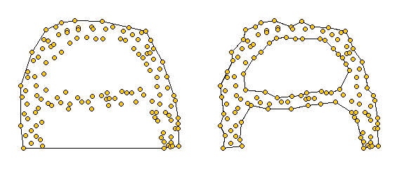
Alpha shapes are generalizations of the convex hull [1]. Convex hulls are well known and widely implemented in GIS systems. Alpha shapes are different in that they capture the shape of a point set. You can watch a great demo of how alpha shapes work on François Bélair’s website “Everything You Always Wanted to Know About Alpha Shapes But Were Afraid to Ask” I borrowed the following pictures from that site:

Alpha shapes for different values of alpha. The left one equals the convex hull of the point set. The right picture represents the alpha shape for a smaller value of alpha

pgRouting comes with an implementation of alpha shapes. There is an alpha shape function: alphashape(sql text) and a convenience wrapper: points_as_polygon(query character varying). The weird thing is that you don’t get to set an alpha value. The only thing supplied to the function is a set of points. Let’s see what kind of results it produces!

Starting point for this experiment is a 10 km catchment zone around node #2699 in my osm road network. Travel costs to nodes are calculated using driving_distance() function. (You can find more information on using this function in Catchment Areas with pgRouting driving_distance().)

CREATE TABLE home_catchment10km AS
SELECT *
   FROM osm_nodes
   JOIN
   (SELECT * FROM driving_distance('
      SELECT gid AS id,
          source,
          target,
          meters AS cost
      FROM osm_roads',
      2699,
      10000,
      false,
      false)) AS route
   ON
   osm_nodes.id = route.vertex_id

After costs are calculated, we can create some alpha shapes. The following queries create the table and insert an alpha shape for all points with a cost of less than 1500:

CREATE TABLE home_isodist (id serial, max_cost double precision);
SELECT AddGeometryColumn('home_isodist','the_geom',4326,'POLYGON',2);

INSERT INTO home_isodist (max_cost, the_geom) (
SELECT 1500, ST_SetSRID(the_geom,4326)
FROM 
  points_as_polygon(
    'SELECT id, ST_X(the_geom) AS x, ST_Y(the_geom) AS y FROM home_catchment10km where cost < 1500'));

In previous posts, I’ve created catchment areas by first interpolating a cost raster and creating contours from there. Now, let’s see how the two different approaches compare!

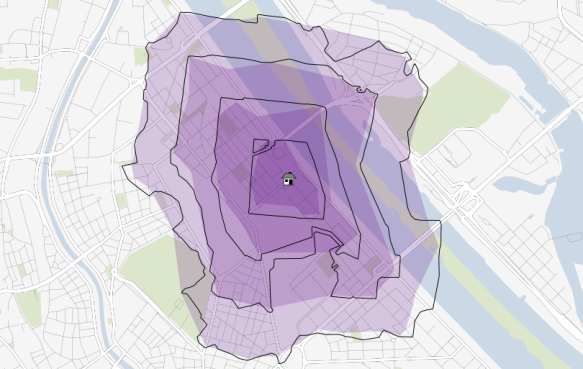
The following picture shows resulting catchment areas for 500, 1000, 1500, and 2000 meters around a central node. Colored areas show the form of pgRouting alpha shape results. Black contours show the results of the interpolation method:

Comparison of pgRouting alpha shapes and interpolation method

At first glance, results look similar enough. Alpha shape results look like a generalized version of interpolation results. I guess that it would be possible to get even closer if the alpha value could be set to a smaller value. The function should then produce a finer, more detailed polygon.

For a general overview about which areas of a network are reachable within certain costs, pgRouting alpha shapes function seems a viable alternative to the interpolation method presented in previous posts. However, the alpha value used by pgRouting seems too big to produce detailed catchment areas.

[1] http://biogeometry.duke.edu/software/alphashapes/

The aim of this post is to describe the steps necessary to calculate routes with pgRouting. In the end, we’ll visualize the results in QGIS.

This guide assumes that you have the following installed and running:

• Postgres with PostGIS and pgAdmin
• QGIS with PostGIS Manager and RT Sql Layer plugins

Installing pgRouting

pgRouting can be downloaded from www.pgrouting.org.

Building from source is covered by pgRouting documentation. If you’re using Windows, download the binaries and copy the .dlls into PostGIS’ lib folder, e.g. C:\Program Files (x86)\PostgreSQL\8.4\lib.

Start pgAdmin and create a new database based on your PostGIS template. (I called mine ‘routing_template’.) Open a Query dialog, load and execute the three .sql files located in your pgRouting download (routing_core.sql, routing_core_wrappers.sql, routing_topology.sql). Congratulations, you now have a pgRouting-enabled database.

Creating a routable road network

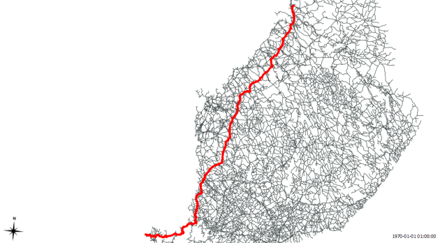
The following description is based on the free road network published by National Land Survey of Finland (NLS). All you get is one Shapefile containing line geometries, a road type attribute and further attributes unrelated to routing.

pgRouting requires each road entry to have a start and an end node id. We’ll create those now:

First step is to load roads.shp into PostGIS. This is easy using PostGIS Manager – Data – Load Data from Shapefile.

Next, we create start and end point geometries. I used a view:

CREATE OR REPLACE VIEW road_ext AS
   SELECT *, startpoint(the_geom), endpoint(the_geom)
   FROM road;

Now, we create a table containing all the unique network nodes (start and end points) and we’ll also give them an id:

CREATE TABLE node AS
   SELECT row_number() OVER (ORDER BY foo.p)::integer AS id,
          foo.p AS the_geom
   FROM (
      SELECT DISTINCT road_ext.startpoint AS p FROM road_ext
      UNION
      SELECT DISTINCT road_ext.endpoint AS p FROM road_ext
   ) foo
   GROUP BY foo.p;

Finally, we can combine our road_ext view and node table to create the routable network table:

CREATE TABLE network AS
   SELECT a.*, b.id as start_id, c.id as end_id
   FROM road_ext AS a
      JOIN node AS b ON a.startpoint = b.the_geom
      JOIN node AS c ON a.endpoint = c.the_geom

(This can take a while.)

I recommend adding a spatial index to the resulting table.

Calculating shortest routes

Let’s try pgRouting’s Shortest Path Dijkstra method. The following query returns the route from node #1 to node #5110:

SELECT * FROM shortest_path('
   SELECT gid AS id,
          start_id::int4 AS source,
          end_id::int4 AS target,
          shape_leng::float8 AS cost
   FROM network',
1,
5110,
false,
false)

Final step: Visualization

With RT Sql Layer plugin, we can visualize the results of a query. The results will be loaded as a new layer. The query has to contain both geometry and a unique id. Therefore, we’ll join the results of the previous query with the network table containing the necessary geometries.

SELECT *
   FROM network
   JOIN
   (SELECT * FROM shortest_path('
      SELECT gid AS id,
          start_id::int4 AS source,
          end_id::int4 AS target,
          shape_leng::float8 AS cost
      FROM network',
      1,
      5110,
      false,
      false)) AS route
   ON
   network.gid = route.edge_id

In my case, this is how the result looks like:

Route from node #1 to node #5110

pgRouting has become even more powerful: A DARP (Dial-a-Ride-Problem) solver is now available in the “darp branch” of the pgRouting repository.

The Dial-a-Ride Problem (DARP) solver tries to minimize transportation cost while satisfying customer service level constraints (time windows violation, waiting and travelling times) and fleet constraints (number of cars and capacity, as well as depot location).

Documentation can be found at www.pgrouting.org/docs.

Today, Alexander Bruy announced a new QGIS plugin called RoadGraph. It is a C++ plugin that calculates the shortest path between two points on any polyline layer (e.g. Openstreetmap shapefiles).

More information can be found at GIS-Lab.

Binary files are available for Windows and Linux:

• Windows: http://svn.gis-lab.info/road-graph/binary/roadgraphplugin.dll (MD5 sum:
  888c0ddf08384dde45a7e16ffeee6f8c roadgraphplugin.dll)
• Linux: http://svn.gis-lab.info/road-graph/binary/libroadgraphplugin.so (MD5 sum:  f48a317381c8d0ef5098f1918f835ca9 libroadgraphplugin.so)

Read on: “Travelling through Brazil with Quantum GIS”