Context
Since last year we (the QGIS communtity) have been using QGIS-Server-PerfSuite to run performance tests on a daily basis. This way, we’re able to monitor and avoid regressions according to some test scenarios for several QGIS Server releases (currently 2.18, 3.4, 3.6 and master branches). However, there are still many questions about performance from a general point of view:
- What is the performance of QGIS Server compared to QGIS Desktop?
- What are the implications of feature simplification for polygons and lines?
- Does the symbology have a strong impact on performance and in which proportion?
Of course, it’s a broad and complex topic because of the numerous possibilities offered by the rendering engine of QGIS. In this article we’ll look at typical use cases with geometries coming from a PostgreSQL database.
Methodology
The first way to monitor performance is to measure the rendering time. To do so, the Map canvas refreshis activated in the Settings of QGIS Desktop. In this way we can get the rendering time from within the Rendering tab of log messages in QGIS Desktop, as well as from log messages written by QGIS Server.

The rendering time retrieved with this method allows to get the total amount of time spent in rendering for each layer (see the source code).
But in the case of QGIS Server another interesting measure is the total time spent for a specific request, which may be read from log messages too. There are indeed more operations achieved for a single WMS request than a simple rendering in QGIS Desktop:
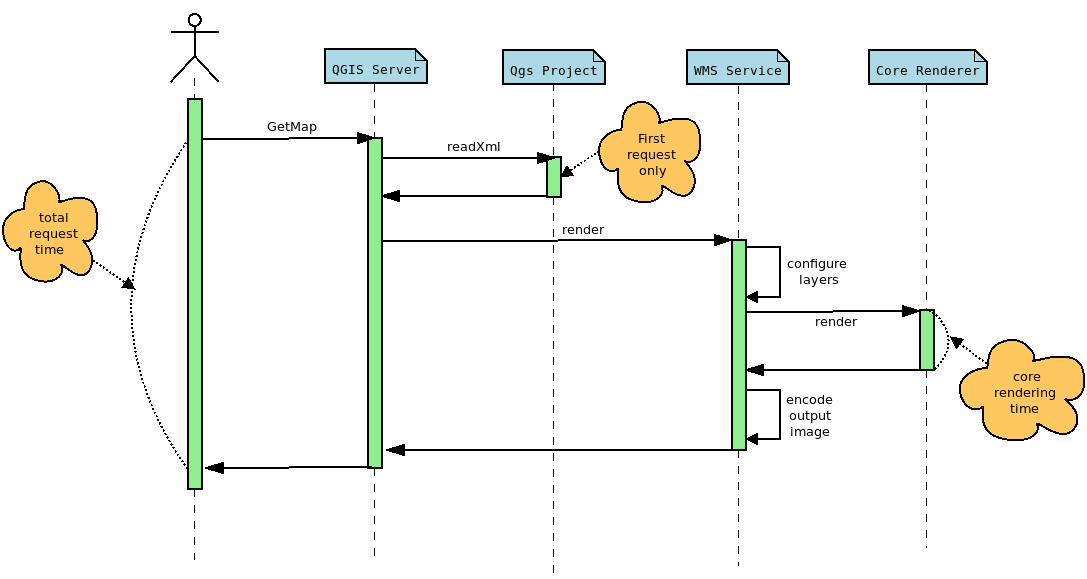
The rendering time extracted from QGIS Desktop corresponds to the core rendering time displayed in the sequence diagram above. Moreover, to be perfectly comparable, the rendering engine must be configured in the same way in both cases. In this way, and thanks to PyQGIS API, we can retrieve the necessary information from the Python console in QGIS Desktop, like the extent or the canvas size, in order to configure the GetMap WMS request with the appropriate WIDTH,, HEIGHT , and BBOX parameters.
Another way to examine the performance is to use a profiler in order to inspect stack traces. These traces may be represented as a FlameGraph. In this case, debug symbols are necessary, meaning that the rendering time is not representative anymore. Indeed, QGIS has to be compiled in Debug mode.
Polygons
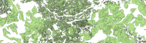
For these tests we use the same dataset as that for the daily performance tests, which is a layer of polygons with 282,776 features.

Feature simplification deactivated
Let’s first have a look at the rendering time and the FlameGraph when the simplification is deactivated. In QGIS Desktop, the mean rendering time is 2591 ms. Using to the PyQGIS API we are able to get the extent and the size of the map to render the map again but using a GetMap WMS request this time.
In this case, the rendering time is 2469 ms and the total request time is 2540 ms. For the record, the first GetMap request is ignored because in this case, the whole QGIS project is read and cached, meaning that the total request time is much higher. But according to those results, the rendering time for QGIS Desktop and QGIS Server are utterly similar, which makes sense considering that the same rendering engine is used, but it is still very reassuring :).
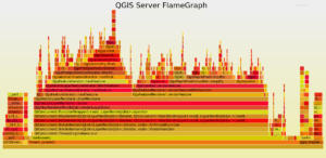
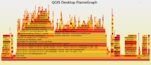
Now, let’s take a look to the FlameGraph to detect where most of the time is spent.
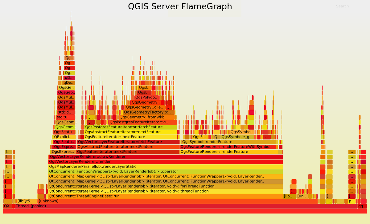
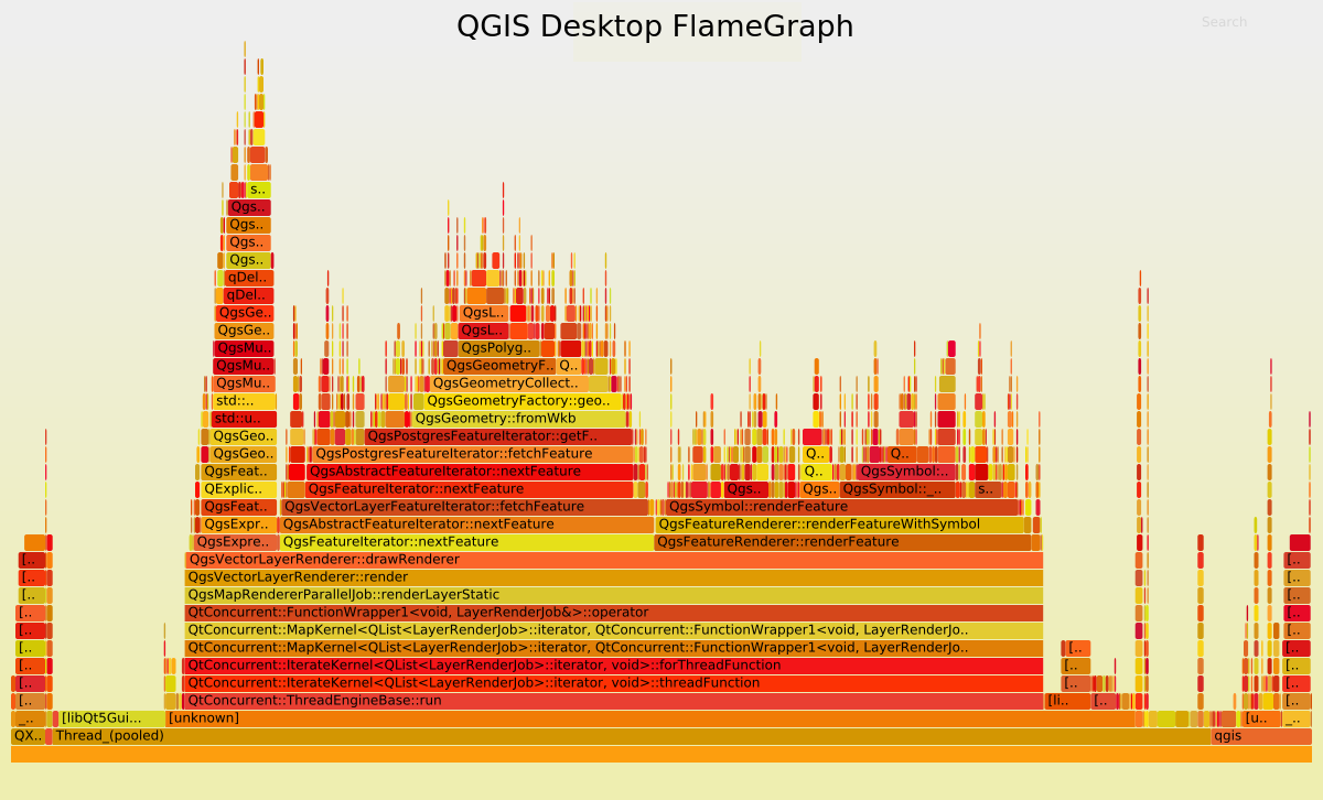
Undoubtedly the FlameGraph’s are similar in both cases, meaning that if we want to improve the performance of QGIS Server we need to improve the performance of the core rendering engine, also used in QGIS Desktop. In our case the main method is QgsMapRendererParallelJob::renderLayerStatic where most of the time is spent in:
| Methods |
Desktop % |
Server % |
| QgsExpressionContext::setFeature |
6.39 |
6.82 |
| QgsFeatureIterator::nextFeature |
28.77 |
28.41 |
| QgsFeatureRenderer::renderFeature |
29.01 |
27.05 |
Basically, it may be simplified like:
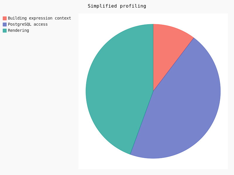
Clearly, the rendering takes about 30% of the total amount of time. In this case geometry simplification could potentially help.
Feature simplification activated
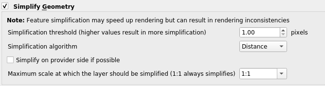
Geometry simplification, available for both polygons and lines layers, may be activated and configured through layer’s Properties in the Rendering tab. Several parameters may be set:
- Simplification may be deactivated
- Threshold for a more drastic simplification
- Algorithm
- Provider simplification
- Scale
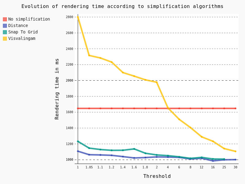
Once the simplification activated, we varied the threshold as well as the algorithm in order to detect performance jumps:
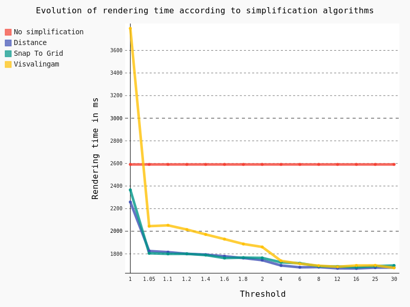
The following conclusions can be drawn:
- The Visvalingam algorithm should be avoided because it begins to be efficient with a high threshold, meaning a significant lack of precision in geometries
- The ideal threshold for Snap To Grid and Distance algorithms seems to be 1.05. Indeed, considering that it’s a very low threshold, the precision of geometries is still pretty good for a major improvement in rendering time though
For now, these tests have been run on the full extent of the layer. However, we still have a Maximum scale parameter to test, so we’ve decreased the scale of the layer:
And in this case, results are pretty interesting too:
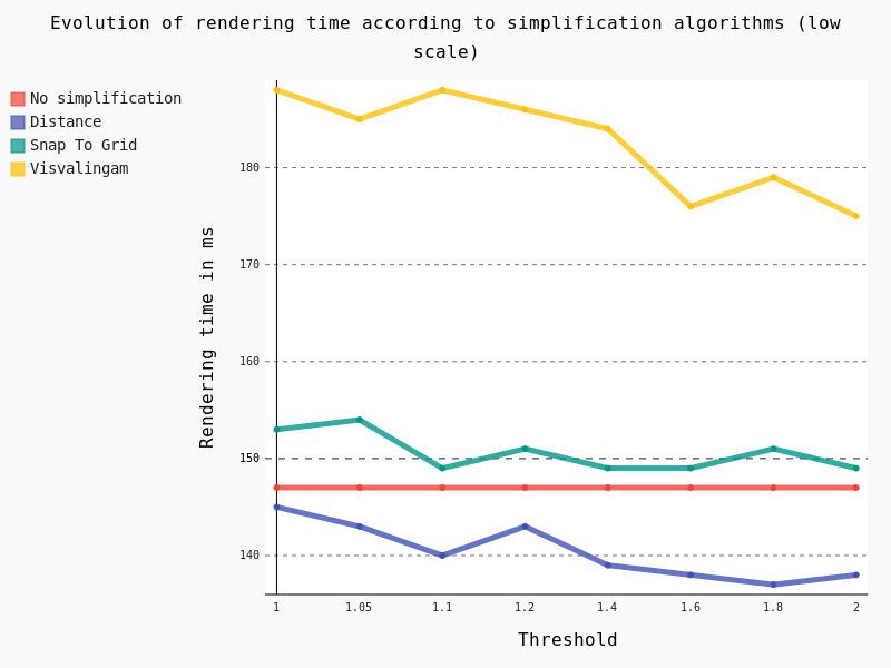
Several conclusions can be drawn:
- Visvalingam algorithm should be avoided at low scale too
- Snap To Grid seems counter-productive at low scale
- Distance algorithm seems to be a good option
Lines
For these tests we also use the same dataset as that for daily performance tests, which is a layer of lines with 125,782 features.

Feature simplification activated
In the same way as for polygons we have tested the effect of the geometric simplification on the rendering time, as well as algorithms and thresholds:
In this case we have exactly the same conclusion as for polygons: the Distance algorithm should be preferred with a threshold of 1.05.
For QGIS Server the mean rendering time is about 1180 ms with geometry simplification compared to 1108 ms for QGIS Desktop, which is totally consistent. And looking at the FlameGraph we note that once again most of the time is spent in accessing the PostgreSQL database (about 30%) and rendering features (about 40%).
Symbology
Another parameter which has an obvious impact on performance is the symbology used to draw the layers. Some features are known to be time consuming, but we’ve felt that a a thorough study was necessary to verify it.
Firstly, we’ve studied the influence of the width as well as the Single Symbol type on the rendering time.
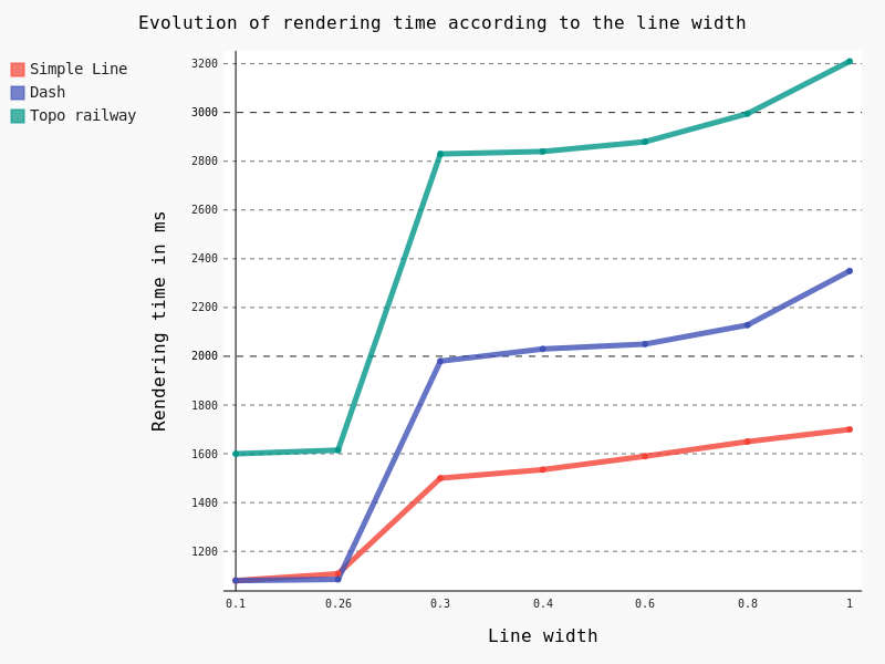 Some points are noteworthy:
– Simple Line is clearly the less time consuming
– Beyond the default 0.26 line width, rendering time begins to raise consequently with a clear jump in performance
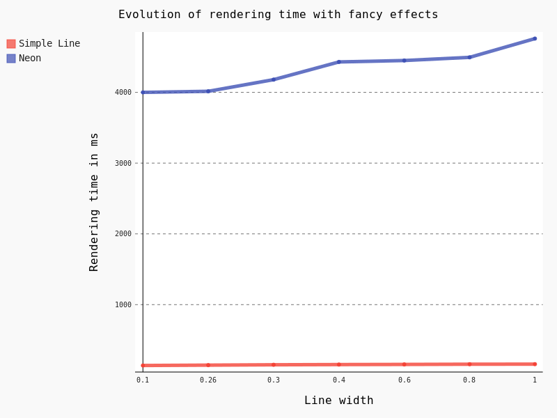
Another interesting feature is the Draw effects option, allowing to add some fancy effects (shadow, glow, …).
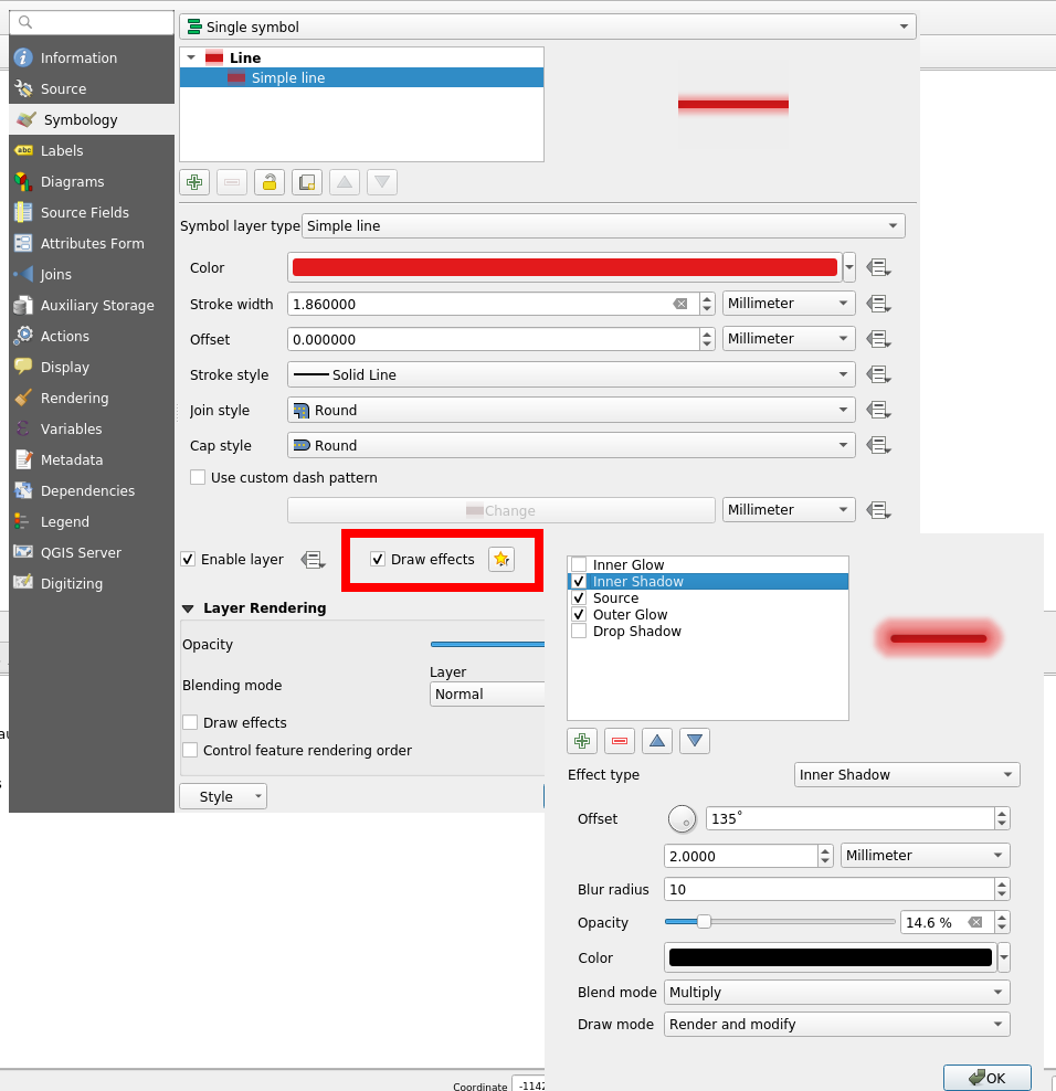
However, this feature is known to be particularly CPU consuming. Actually, rendering all the 125,782 lines took so long that we had to to change to a lower scale, with just some a few dozen lines. Results are unequivocal:
The last thing we wanted to test for symbology is the effect of the Categorized classification. Here are the results for some classifications with geometry simplification activated:
- No classification: 1108 ms
- A simple classification using the column “classification” (8 symbols): 1148 ms
- A classification based on a stupid expression “classification x 3″ (8 symbols): 1261 ms
- A classification based on string comparison “toponyme like ‘Ruisseau*'” (2 symbols): 1380 ms
- A classification with a specific width line for each category (8 symbols): 1850 ms
Considering that a simple classification does not add an excessive extra-cost, it seems that the classification process itself is not very time consuming. However, as soon as an expression is used, we can observe a slight jump in performance.
Labeling
Another important part to study regarding performance is labeling and the underlying positioning. For this test we decreased the scale and varied the Placement parameter without tuning anything.
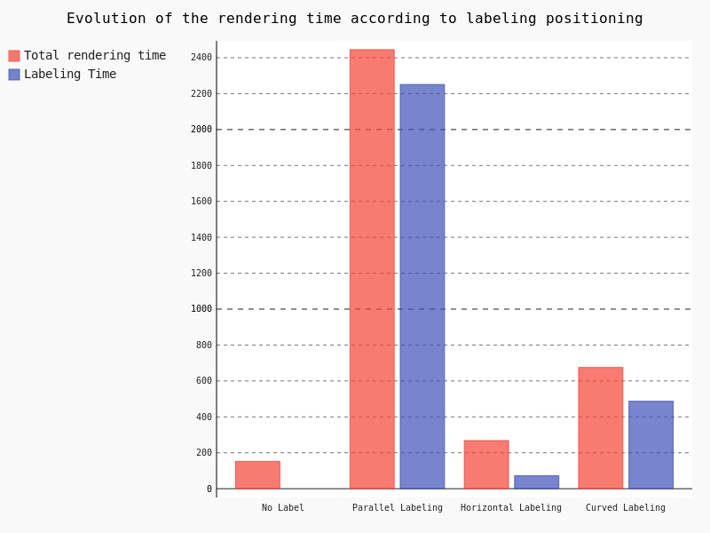
Clearly, the parallel labeling is much more time consuming than the other placements. However, as previously stated, we used the default parameters for each positioning, meaning that the number of labels really drawn on the map differs from a placement to another.
Points
The last kind of geometries we have to study is points. Similarly to polygons and lines, we used the same dataset as that of performance tests, that is a layer with 435588 points.
In the case of points geometries geometry simplification is of course not available. So we are going to focus on symbology and the impact of marker size.
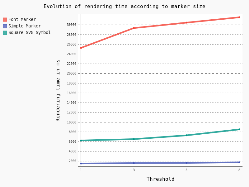
Obviously Font Marker must be used carefully because of the underlying jump in performance, as well as SVG Symbols. Moreover, contrary to Simple Marker, an increase of the size implies a drastic augmentation in time rendering.
General conclusion
Based on this factual study, several conclusions can be drawn.
Globally, FlameGraph for QGIS Desktop and QGIS Server are completely similar as well as rendering time.
It means that if we want to improve the performance of QGIS Server, we have to work on the desktop configuration and the rendering engine of the QGIS core library.
Extracting generic conclusions from our tests is very difficult, because it clearly depends on the underlying data. But let’s try to suggest some recommendations :).
Firstly, geometry simplification seems pretty efficient with lines and polygons as soon as the algorithm is chosen cautiously, and as long as your features include many vertices. It seems that the Distance algorithm with a 1.05 threshold is a good choice, with both high and low scale. However, it’s not a magic solution!
Secondly, a special care is needed with regards to symbology. Indeed, in some cases, a clear jump in performance is notable. For example, fancy effects and Font Marker / SVG Symbol have to be used with caution if you’re picky on rendering time.
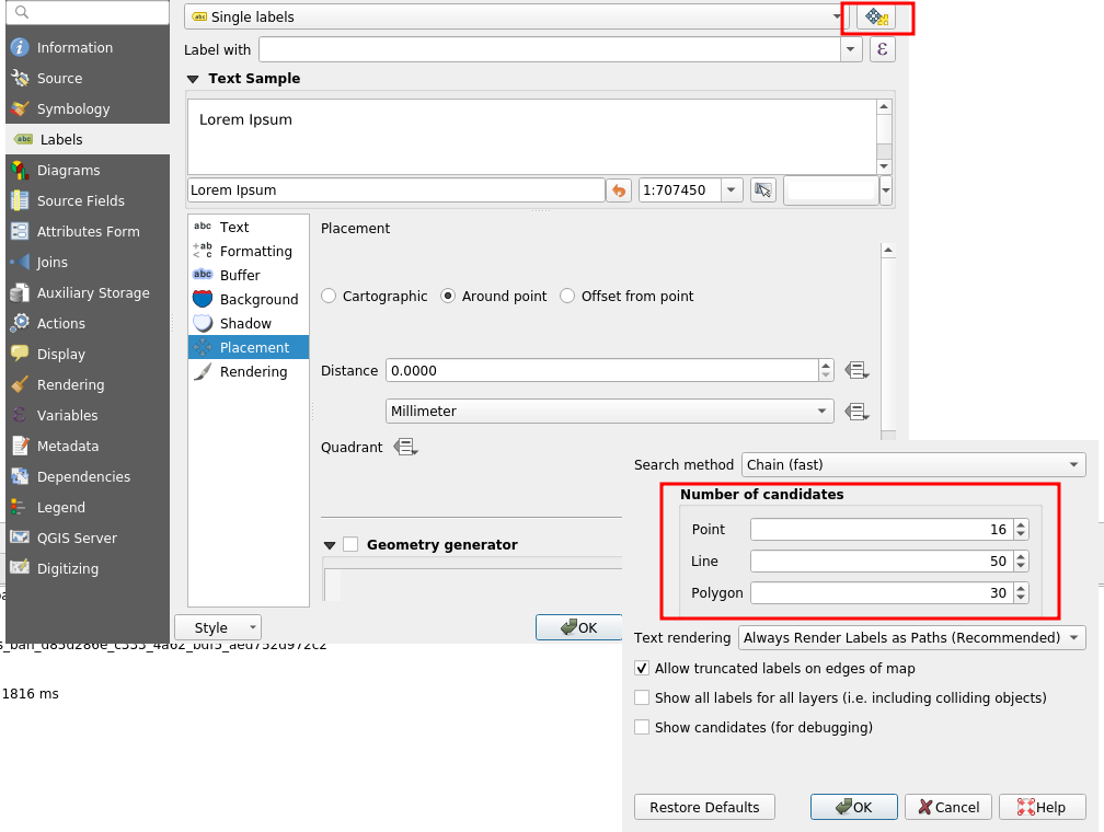
Thirdly, we have to be aware of the extra cost caused by labeling, especially the Parallel placement for line geometries. On this subject, a not very well-known parameter allows to drastically reduce labeling time: the PAL candidates option. Actually, we may decrease the labeling time by reducing the number of candidates. For an explicit use case, you can take a look at the daily reports.
In any case, improving server performance in a substantial way means improving the QGIS core library directly.
Especially, we noticed thanks to FlameGraph that most of the time is spent in drawing features and managing the data from the PostgreSQL database. By the way, a legitimate question is: “How much time do we spend on waiting for the database?”. To be continued 
If you hit performance issues on your specific configuration or want to improve QGIS awesomeness, we provide a unique QGIS support offer at http://qgis.oslandia.com/ thanks to our team of specialists!


 You will probably interact first with our pre-sales engineer Bertrand Parpoil. He leads Geographical Information System projects for 15 years for large corporations, public administrations or hi-tech SME. Bertrand will listen to your needs and explore your use cases, to offer you the best set of services.
  Régis Haubourg also takes part in the first steps of projects to analyze your usages and improve them. GIS Expert, he knows QGIS by heart and will make the most of its capabilities. As QGIS Community Manager at Oslandia, he is very active in the QGIS community of developers and contributors. He is president of the Francophone OSGeo local chapter ( OSGeo-fr ), QGIS voting member, organizes the French QGIS day conference in Montpellier, and participates to QGIS community meetings. Before joining Oslandia, he led the migration to QGIS and PostGIS at the Adour-Garonne Water Agency, and now guides our clients with their GIS migrations to OpenSource solutions. Régis is also a great asset when working on water, hydrology and other specific thematic subjects.
 Loïc Bartoletti develops QGIS, specializing in features corresponding to his fields of interests : network management, topography, urbanism, architecture… We find him contributing to advanced vector editing in QGIS, writing Python plugins, namely for DICT management. Pushing CAD and migrations from CAD tools to GIS and QGIS is one of his major goals. He will develop your custom applications, combining technical expertise and functional competences. When bored, Loïc packages software on FreeBSD.
 Vincent Mora is senior developer in Python and C++, as well as PostGIS expert. He has a strong experience in numerical simulation. He likes coupling GIS (PostGIS, QGIS) with 3D numerical computing for risk management or production optimization. Vincent is an official QGIS committer and can directly integrate your needs into the core of the software. He is also GDAL committer and optimizes low-level layers of your applications. Among numerous activities, Vincent serves as lead developer of the development team for
 Hugo Mercier is an officiel QGIS committer too for several years. He regularly talks in international conferences on PostGIS, QGIS and other OpenSource GIS softwares. He will implement your needs with new QGIS features, develop innovative plugins ( like
 Paul Blottière completes our QGIS committers : very active on core development, Paul has refactored the QGIS server component to bring it to an industry-grade quality level. He also designed and implemented
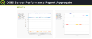
 Julien Cabièces recently joined Oslandia, and quickly dived into QGIS : he contributes to the core of this Desktop GIS, on the server component, as well as applications linked to numerical simulation. Coming from a satellite imagery company with industrial applications, he uses his flexibility to answer all your needs. He brings quality and professionalism to your projects, minimizing risks for large production deployments.
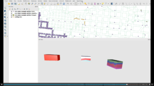
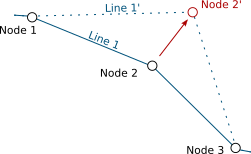
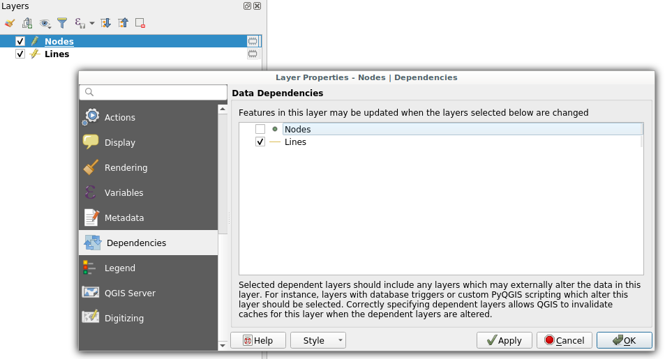 Dependencies configuration: Lines layer will be refreshed whenever Nodes layer is modified
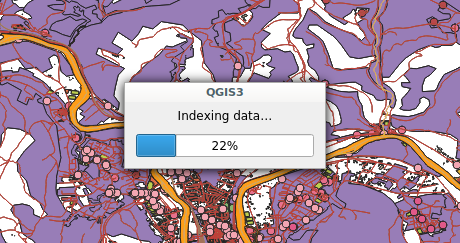 Snap indexing dialog
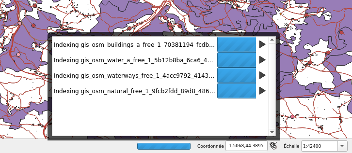 4 layers snap index being built in parallel