


QGIS Versioning now supports foreign keys!
QGIS-versioning is a QGIS and PostGIS plugin dedicated to data versioning and history management. It supports :
- Keeping full table history with all modifications
- Transparent access to current data
- Versioning tables with branches
- Work offline
- Work on a data subset
- Conflict management with a GUI
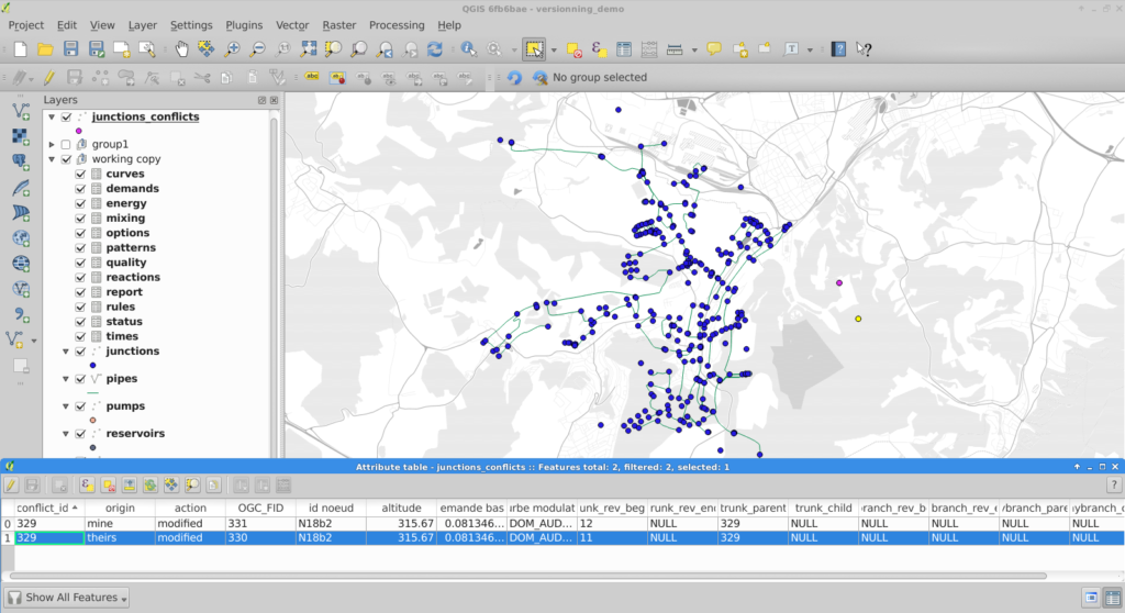
QGIS versioning conflict management
In a previous blog article we detailed how QGIS versioning can manage data history, branches, and work offline with PostGIS-stored data and QGIS. We recently added foreign key support to QGIS versioning so you can now historize any complex database schema.
This QGIS plugin is available in the official QGIS plugin repository, and you can fork it on GitHub too !
Foreign key support
TL;DR
When a user decides to historize its PostgreSQL database with QGIS-versioning, the plugin alters the existing database schema and adds new fields in order to track down the different versions of a single table row. Every access to these versioned tables are subsequently made through updatable views in order to automatically fill in the new versioning fields.
Up to now, it was not possible to deal with primary keys and foreign keys : the original tables had to be constraints-free. This limitation has been lifted thanks to this contribution.
To make it simple, the solution is to remove all constraints from the original database and transform them into a set of SQL check triggers installed on the working copy databases (SQLite or PostgreSQL). As verifications are made on the client side, it’s impossible to propagate invalid modifications on your base server when you “commit” updates.
Behind the curtains
When you choose to historize an existing database, a few fields are added to the existing table. Among these fields, versioning_ididentifies one specific version of a row. For one existing row, there are several versions of this row, each with a different versioning_id but with the same original primary key field. As a consequence, that field cannot satisfy the unique constraint, so it cannot be a key, therefore no foreign key neither.
We therefore have to drop the primary key and foreign key constraints when historizing the table. Before removing them, constraints definitions are stored in a dedicated table so that these constraints can be checked later.
When the user checks out a specific table on a specific branch, QGIS-versioning uses that constraint table to build constraint checking triggers in the working copy. The way constraints are built depends on the checkout type (you can checkout in a SQLite file, in the master PostgreSQL database or in another PostgreSQL database).
What do we check ?
That’s where the fun begins ! The first thing we have to check is key uniqueness or foreign key referencing an existing key on insert or update. Remember that there are no primary key and foreign key anymore, we dropped them when activating historization. We keep the term for better understanding.
You also have to deal with deleting or updating a referenced row and the different ways of propagating the modification : cascade, set default, set null, or simply failure, as explained in PostgreSQL Foreign keys documentation .
Nevermind all that, this problem has been solved for you and everything is done automatically in QGIS-versioning. Before you ask, yes foreign keys spanning on multiple fields are also supported.
What’s new in QGIS ?
You will get a new message you probably already know about, when you try to make an invalid modification committing your changes to the master database
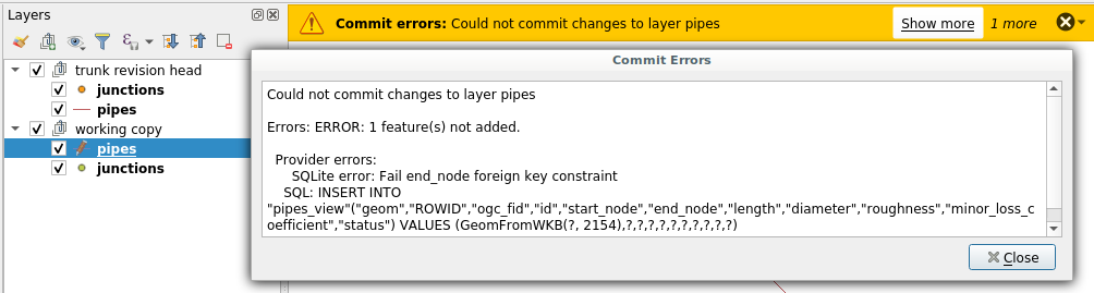
Error when foreign key constraint is violated
Partial checkout
One existing Qgis-versioning feature is partial checkout. It allows a user to select a subset of data to checkout in its working copy. It avoids downloading gigabytes of data you do not care about. You can, for instance, checkout features within a given spatial extent.
So far, so good. But if you have only a part of your data, you cannot ensure that modifying a data field as primary key will keep uniqueness. In this particular case, QGIS-versioning will trigger errors on commit, pointing out the invalid rows you have to modify so the unique constraint remains valid.
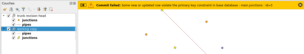
Error when committing non unique key after a partial checkout
Tests
There is a lot to check when you intend to replace the existing constraint system with your own constraint system based on triggers. In order to ensure QGIS-Versioning stability and reliability, we put some special effort on building a test set that cover all use cases and possible exceptions.
What’s next
There is now no known limitations on using QGIS-versioning on any of your database. If you think about a missing feature or just want to know more about QGIS and QGIS-versioning, feel free to contact us at [email protected]. And please have a look at our support offering for QGIS.
Many thanks to eHealth Africa who helped us develop these new features. eHealth Africa is a non-governmental organization based in Nigeria. Their mission is to build stronger health systems through the design and implementation of data-driven solutions.

OSM data quality assessment: producing map to illustrate data quality
At Oslandia, we like working with Open Source tool projects and handling Open (geospatial) Data. In this article series, we will play with the OpenStreetMap (OSM) map and subsequent data. Here comes the eighth article of this series, dedicated to the OSM data quality evaluation, through production of new maps.
1 Description of OSM element
1.1 Element metadata extraction
As mentionned in a previous article dedicated to metadata extraction, we have to focus on element metadata itself if we want to produce valuable information about quality. The first questions to answer here are straightforward: what is an OSM element? and how to extract its associated metadata?. This part is relatively similar to the job already done with users.
We know from previous analysis that an element is created during a changeset by a given contributor, may be modified several times by whoever, and may be deleted as well. This kind of object may be either a “node”, a “way” or a “relation”. We also know that there may be a set of different tags associated with the element. Of course the list of every operations associated to each element is recorded in the OSM data history. Let’s consider data around Bordeaux, as in previous blog posts:
import pandas as pd
elements = pd.read_table('../src/data/output-extracts/bordeaux-metropole/bordeaux-metropole-elements.csv', parse_dates=['ts'], index_col=0, sep=",")
elements.head().T
   elem        id  version  visible         ts    uid  chgset
0  node  21457126        2    False 2008-01-17  24281  653744
1  node  21457126        3    False 2008-01-17  24281  653744
2  node  21457126        4    False 2008-01-17  24281  653744
3  node  21457126        5    False 2008-01-17  24281  653744
4  node  21457126        6    False 2008-01-17  24281  653744
This short description helps us to identify some basic features, which are built in the following snippets. First we recover the temporal features:
elem_md = (elements.groupby(['elem', 'id'])['ts']
            .agg(["min", "max"])
            .reset_index())
elem_md.columns = ['elem', 'id', 'first_at', 'last_at']
elem_md['lifespan'] = (elem_md.last_at - elem_md.first_at)/pd.Timedelta('1D')
extraction_date = elements.ts.max()
elem_md['n_days_since_creation'] = ((extraction_date - elem_md.first_at)
                                  / pd.Timedelta('1d'))
elem_md['n_days_of_activity'] = (elements
                              .groupby(['elem', 'id'])['ts']
                              .nunique()
                              .reset_index())['ts']
elem_md = elem_md.sort_values(by=['first_at'])
                                    213418
elem                                  node
id                               922827508
first_at               2010-09-23 00:00:00
last_at                2010-09-23 00:00:00
lifespan                                 0
n_days_since_creation                 2341
n_days_of_activity                       1
Then the remainder of the variables, e.g. how many versions, contributors, changesets per elements:
    elem_md['version'] = (elements.groupby(['elem','id'])['version']
                          .max()
                          .reset_index())['version']
    elem_md['n_chgset'] = (elements.groupby(['elem', 'id'])['chgset']
                           .nunique()
                           .reset_index())['chgset']
    elem_md['n_user'] = (elements.groupby(['elem', 'id'])['uid']
                         .nunique()
                         .reset_index())['uid']
    osmelem_last_user = (elements
                         .groupby(['elem','id'])['uid']
                         .last()
                         .reset_index())
    osmelem_last_user = osmelem_last_user.rename(columns={'uid':'last_uid'})
    elements = pd.merge(elements, osmelem_last_user,
                       on=['elem', 'id'])
    elem_md = pd.merge(elem_md,
                       elements[['elem', 'id', 'version', 'visible', 'last_uid']],
                       on=['elem', 'id', 'version'])
    elem_md = elem_md.set_index(['elem', 'id'])
    elem_md.sample().T
elem                                  node
id                              1340445266
first_at               2011-06-26 00:00:00
last_at                2011-06-27 00:00:00
lifespan                                 1
n_days_since_creation                 2065
n_days_of_activity                       2
version                                  2
n_chgset                                 2
n_user                                   1
visible                              False
last_uid                            354363
As an illustration we have above an old two-versionned node, no more visible on the OSM website.
1.2 Characterize OSM elements with user classification
This set of features is only descriptive, we have to add more information to be able to characterize OSM data quality. That is the moment to exploit the user classification produced in the last blog post!
As a recall, we hypothesized that clustering the users permits to evaluate their trustworthiness as OSM contributors. They are either beginners, or intermediate users, or even OSM experts, according to previous classification.
Each OSM entity may have received one or more contributions by users of each group. Let’s say the entity quality is good if its last contributor is experienced. That leads us to classify the OSM entities themselves in return!
How to include this information into element metadata?
We first need to recover the results of our clustering process.
user_groups = pd.read_hdf("../src/data/output-extracts/bordeaux-metropole/bordeaux-metropole-user-kmeans.h5", "/individuals")
user_groups.head()
           PC1       PC2       PC3       PC4       PC5       PC6  Xclust
uid
1626 -0.035154  1.607427  0.399929 -0.808851 -0.152308 -0.753506       2
1399 -0.295486 -0.743364  0.149797 -1.252119  0.128276 -0.292328       0
2488  0.003268  1.073443  0.738236 -0.534716 -0.489454 -0.333533       2
5657 -0.889706  0.986024  0.442302 -1.046582 -0.118883 -0.408223       4
3980 -0.115455 -0.373598  0.906908  0.252670  0.207824 -0.575960       5
As a remark, there were several important results to save after the clustering process; we decided to serialize them into a single binary file. Pandas knows how to manage such file, that would be a pity not to take advantage of it!
We recover the individuals groups in the eponym binary file tab (column Xclust), and only have to join it to element metadata as follows:
elem_md = elem_md.join(user_groups.Xclust, on='last_uid')
elem_md = elem_md.rename(columns={'Xclust':'last_uid_group'})
elem_md.reset_index().to_csv("../src/data/output-extracts/bordeaux-metropole/bordeaux-metropole-element-metadata.csv")
elem_md.sample().T
elem                                  node
id                              1530907753
first_at               2011-12-04 00:00:00
last_at                2011-12-04 00:00:00
lifespan                                 0
n_days_since_creation                 1904
n_days_of_activity                       1
version                                  1
n_chgset                                 1
n_user                                   1
visible                               True
last_uid                             37548
last_uid_group                           2
From now, we can use the last contributor cluster as an additional information to generate maps, so as to study data quality…
Wait… There miss another information, isn’t it? Well yes, maybe the most important one, when dealing with geospatial data: the location itself!
1.3 Recover the geometry information
Even if Pyosmium library is able to retrieve OSM element geometries, we realized some tests with an other OSM data parser here: osm2pgsql.
We can recover geometries from standard OSM data with this tool, by assuming the existence of an osm database, owned by user:
osm2pgsql -E 27572 -d osm -U user -p bordeaux_metropole --hstore ../src/data/raw/bordeaux-metropole.osm.pbf
We specify a France-focused SRID (27572), and a prefix for naming output databases point, line, polygon and roads.
We can work with the line subset, that contains the physical roads, among other structures (it roughly corresponds to the OSM ways), and build an enriched version of element metadata, with geometries.
First we can create the table bordeaux_metropole_geomelements, that will contain our metadata…
DROP TABLE IF EXISTS bordeaux_metropole_elements;
DROP TABLE IF EXISTS bordeaux_metropole_geomelements;
CREATE TABLE bordeaux_metropole_elements(
       id int,
       elem varchar,
       osm_id bigint,
       first_at varchar,
       last_at varchar,
       lifespan float,
       n_days_since_creation float,
       n_days_of_activity float,
       version int,
       n_chgsets int,
       n_users int,
       visible boolean,
       last_uid int,
       last_user_group int
);
…then, populate it with the data accurate .csv file…
COPY bordeaux_metropole_elements
FROM '/home/rde/data/osm-history/output-extracts/bordeaux-metropole/bordeaux-metropole-element-metadata.csv'
WITH(FORMAT CSV, HEADER, QUOTE '"');
…and finally, merge the metadata with the data gathered with osm2pgsql, that contains geometries.
SELECT l.osm_id, h.lifespan, h.n_days_since_creation,
h.version, h.visible, h.n_users, h.n_chgsets,
h.last_user_group, l.way AS geom
INTO bordeaux_metropole_geomelements
FROM bordeaux_metropole_elements as h
INNER JOIN bordeaux_metropole_line as l
ON h.osm_id = l.osm_id AND h.version = l.osm_version
WHERE l.highway IS NOT NULL AND h.elem = 'way'
ORDER BY l.osm_id;
Wow, this is wonderful, we have everything we need in order to produce new maps, so let’s do it!
2 Keep it visual, man!
From the last developments and some hypothesis about element quality, we are able to produce some customized maps. If each OSM entities (e.g. roads) can be characterized, then we can draw quality maps by highlighting the most trustworthy entities, as well as those with which we have to stay cautious.
In this post we will continue to focus on roads within the Bordeaux area. The different maps will be produced with the help of Qgis.
2.1 First step: simple metadata plotting
As a first insight on OSM elements, we can plot each OSM ways regarding simple features like the number of users who have contributed, the number of version or the element anteriority.
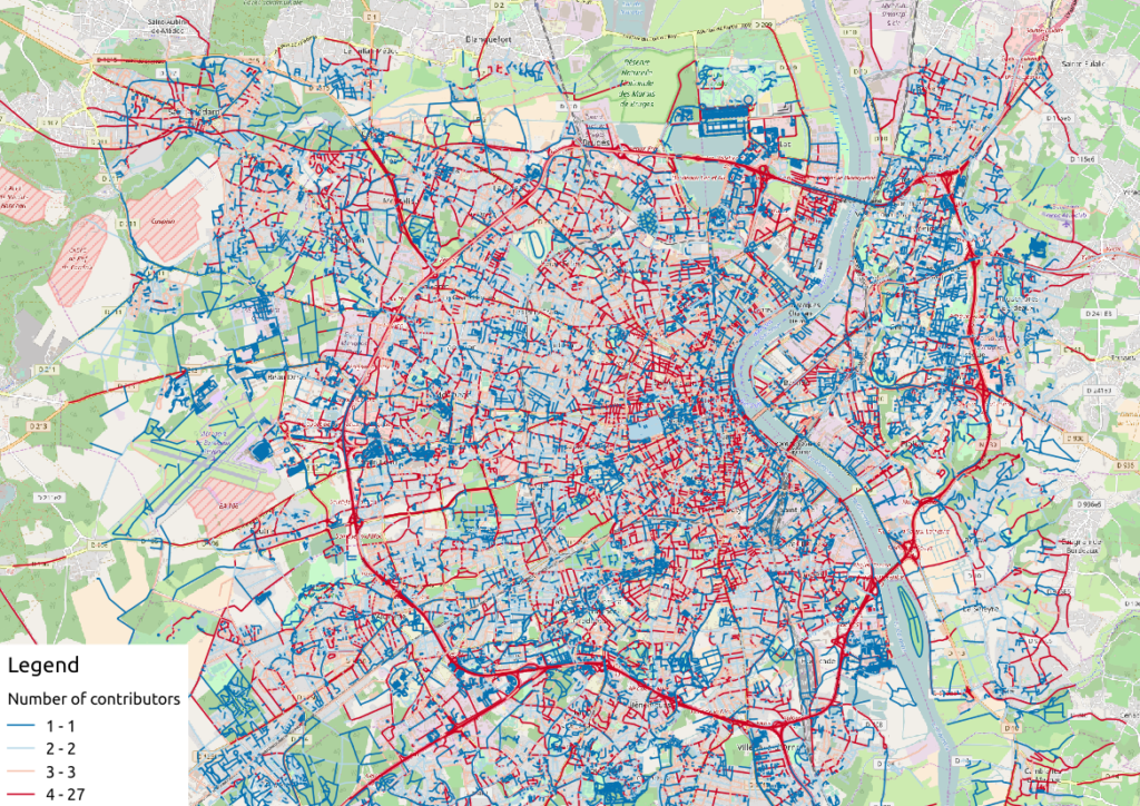
Figure 1: Number of active contributors per OSM way in Bordeaux
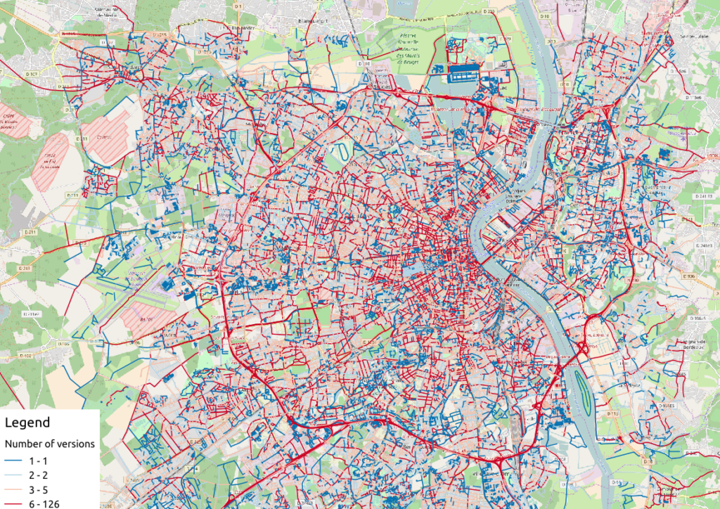
Figure 2: Number of versions per OSM way in Bordeaux
With the first two maps, we see that the ring around Bordeaux is the most intensively modified part of the road network: more unique contributors are implied in the way completion, and more versions are designed for each element. Some major roads within the city center present the same characteristics.

Figure 3: Anteriority of each OSM way in Bordeaux, in years
If we consider the anteriority of OSM roads, we have a different but interesting insight of the area. The oldest roads are mainly located within the city center, even if there are some exceptions. It is also interesting to notice that some spatial patterns arise with temporality: entire neighborhoods are mapped within the same anteriority.
2.2 More complex: OSM data merging with alternative geospatial representations
To go deeper into the mapping analysis, we can use the INSEE carroyed data, that divides France into 200-meter squared tiles. As a corollary OSM element statistics may be aggregated into each tile, to produce additional maps. Unfortunately an information loss will occur, as such tiles are only defined where people lives. However it can provides an interesting alternative illustration.
To exploit such new data set, we have to merge the previous table with the accurate INSEE table. Creating indexes on them is of great interest before running such a merging operation:
CREATE INDEX insee_geom_gist
ON open_data.insee_200_carreau USING GIST(wkb_geometry);
CREATE INDEX osm_geom_gist
ON bordeaux_metropole_geomelements USING GIST(geom);

DROP TABLE IF EXISTS bordeaux_metropole_carroyed_ways;
CREATE TABLE bordeaux_metropole_carroyed_ways AS (
SELECT insee.ogc_fid, count(*) AS nb_ways,
avg(bm.version) AS avg_version, avg(bm.lifespan) AS avg_lifespan,
avg(bm.n_days_since_creation) AS avg_anteriority,
avg(bm.n_users) AS avg_n_users, avg(bm.n_chgsets) AS avg_n_chgsets,
insee.wkb_geometry AS geom
FROM open_data.insee_200_carreau AS insee
JOIN bordeaux_metropole_geomelements AS bm
ON ST_Intersects(insee.wkb_geometry, bm.geom)
GROUP BY insee.ogc_fid
);
As a consequence, we get only 5468 individuals (tiles), a quantity that must be compared to the 29427 roads previously handled… This operation will also simplify the map analysis!
We can propose another version of previous maps by using Qgis, let’s consider the average number of contributors per OSM roads, for each tile:
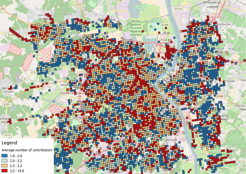
Figure 4: Number of contributors per OSM roads, aggregated by INSEE tile
2.3 The cherry on the cake: representation of OSM elements with respect to quality
Last but not least, the information about last user cluster can shed some light on OSM data quality: by plotting each roads according to the last user who has contributed, we might identify questionable OSM elements!
We simply have to design similar map than in previous section, with user classification information:
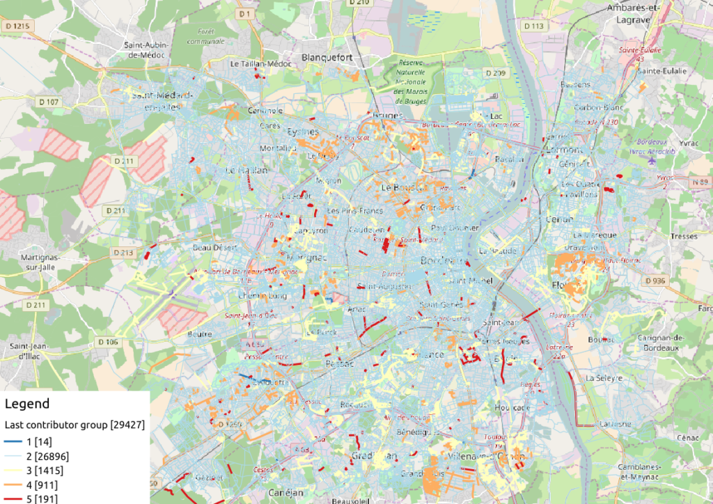
Figure 5: OSM roads around Bordeaux, according to the last user cluster (1: C1, relation experts; 2: C0, versatile expert contributors; 3: C4, recent one-shot way contributors; 4: C3, old one-shot way contributors; 5: C5, locally-unexperienced way specialists)
According to the clustering done in the previous article (be careful, the legend is not the same here…), we can make some additional hypothesis:
- Light-blue roads are OK, they correspond to the most trustful cluster of contributors (91.4% of roads in this example)
- There is no group-0 road (group 0 corresponds to cluster C2 in the previous article)… And that’s comforting! It seems that “untrustworthy” users do not contribute to roads or -more probably- that their contributions are quickly amended.
- Other contributions are made by intermediate users: a finer analysis should be undertaken to decide if the corresponding elements are valid. For now, we can consider everything is OK, even if local patterns seem strong. Areas of interest should be verified (they are not necessarily of low quality!)
For sure, it gives a fairly new picture of OSM data quality!
3 Conclusion
In this last article, we have designed new maps on a small area, starting from element metadata. You have seen the conclusion of our analysis: characterizing the OSM data quality starting from the user contribution history.
Of course some works still have to be done, however we detailed a whole methodology to tackle the problem. We hope you will be able to reproduce it, and to design your own maps!
Feel free to contact us if you are interested in this topic!
