According to the definition of software quality given by french Wikipedia
An overall assessment of quality takes into account external factors, directly observable by the user, as well as internal factors, observable by engineers during code reviews or maintenance work.
I have chosen in this article to only talk about the latter. The quality of software and more precisely QGIS is therefore not limited to what is described here. There is still much to say about:
- Taking user feedback into account,
- the documentation writing process,
- translation management,
- interoperability through the implementation of standards,
- the extensibility using API,
- the reversibility and resilience of the open source model…
These are subjects that we care a lot and deserve their own article.
I will focus here on the following issue: QGIS is free software and allows anyone with the necessary skills to modify the software. But how can we ensure that the multiple proposals for modifications to the software contribute to its improvement and do not harm its future maintenance?
Self-discipline
All developers contributing to QGIS code doesn’t belong to the same organization. They don’t all live in the same country, don’t necessarily have the same culture and don’t necessarily share the same interests or ambitions for the software. However, they share the awareness of modifying a common good and the desire to take care of it.
This awareness transcends professional awareness, the developer not only has a responsibility towards his employer, but also towards the entire community of users and contributors to the software.
This self-discipline is the foundation of the quality of the contributions of software like QGIS.
However, to err is human and it is essential to carry out checks for each modification proposal.
Automatic checks
With each modification proposal (called Pull Request or Merge Request), the QGIS GitHub platform automatically launches a set of automatic checks.
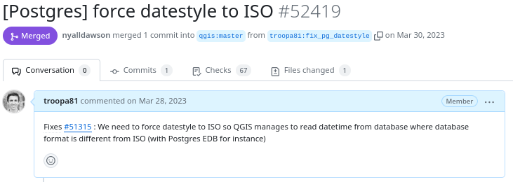
Example of proposed modification
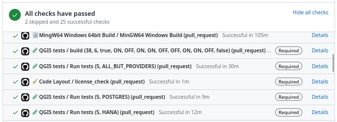
Result of automatic checks on a modification proposal
The first of these checks is to build QGIS on the different systems on which it is distributed (Linux, Windows, MacOS) by integrating the proposed modification. It is inconceivable to integrate a modification that would prevent the application from being built on one of these systems.
The tests
The first problem posed by a proposed modification is the following “How can we be sure that what is going to be introduced does not break what already exists?”
To validate this assertion, we rely on automatic tests. This is a set of micro-programs called tests, which only purpose is to validate that part of the application behaves as expected. For example, there is a test which validates that when the user adds an entry in a data layer, then this entry is then present in the data layer. If a modification were to break this behavior, then the test would fail and the proposal would be rejected (or more likely corrected).
This makes it possible in particular to avoid regressions (they are very often called non-regression tests) and also to qualify the expected behavior.
There are approximately 1.3 Million lines of code for the QGIS application and 420K lines of test code, a ratio of 1 to 3. The presence of tests is mandatory for adding functionality, therefore the quantity of test code increases with the quantity of application code.
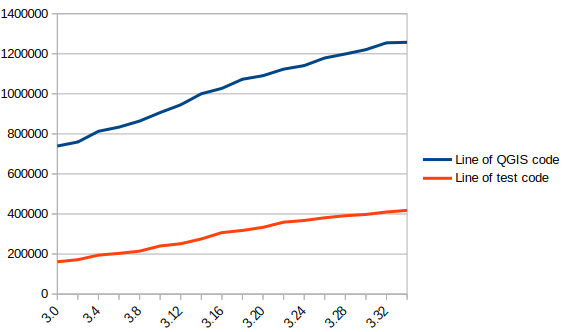
In blue the number of lines of code in QGIS, in red the number of lines of tests
There are currently over 900 groups of automatic tests in QGIS, most of which run in less than 2 seconds, for a total execution time of around 30 minutes.
We also see that certain parts of the QGIS code – the most recent – are better covered by the tests than other older ones. Developers are gradually working to improve this situation to reduce technical debt.
Code checks
Analogous to using a spell checker when writing a document, we carry out a set of quality checks on the source code. We check, for example, that the proposed modification does not contain misspelled words or “banned” words, that the API documentation has been correctly written or that the modified code respects certain formal rules of the programming language.
We recently had the opportunity to add a check based on the clang-tidy tool. The latter relies on the Clang compiler. It is capable of detecting programming errors by carrying out a static analysis of the code.
Clang-tidy is, for example, capable of detecting “narrowing conversions”.

Example of detecting “narrowing conversions”
In the example above, Clang-tidy detects that there has been a “narrowing conversion” and that the value of the port used in the network proxy configuration “may” be corrupted. In this case, this problem was reported on the QGIS issues platform and had to be corrected.
At that time, clang-tidy was not in place. Its use would have made it possible to avoid this anomaly and all the steps which led to its correction (exhaustive description of the issue, multiple exchanges to be able to reproduce it, investigation, correction, review of the modification), meaning a significant amount of human time which could thus have been avoided.
Peer review
A proposed modification that would validate all of the automatic checks described above would not necessarily be integrated into the QGIS code automatically. In fact, its code may be poorly designed or the modification poorly thought out. The relevance of the functionality may be doubtful, or duplicated with another. The integration of the modification would therefore potentially cause a burden for the people in charge of the corrective or evolutionary maintenance of the software.
It is therefore essential to include a human review in the process of accepting a modification.
This is more of a rereading of the substance of the proposal than of the form. For the latter, we favor the automatic checks described above in order to simplify the review process.
Therefore, human proofreading takes time, and this effort is growing with the quantity of modifications proposed in the QGIS code. The question of its funding arises, and discussions are in progress. The QGIS.org association notably dedicates a significant part of its budget to fund code reviews.
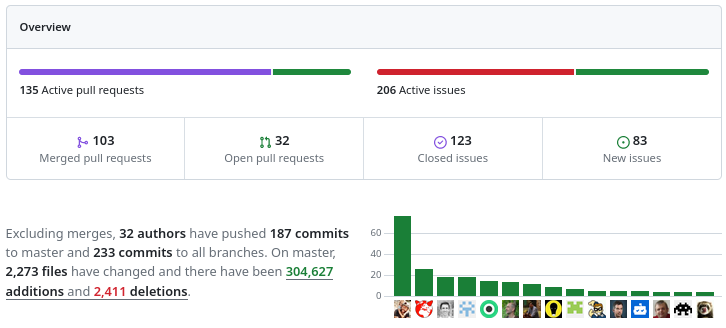
More than 100 modification proposals were reviewed and integrated during the month of December 2023. More than 30 different people contributed. More than 2000 files have been modified.
Therefore the wait for a proofreading can sometimes be long. It is also often the moment when disagreements are expressed. It is therefore a phase which can prove frustrating for contributors, but it is an important and rich moment in the community life of a free project.
To be continued !
As a core QGIS developer, and as a pure player OpenSource company, we believe it is fundamental to be involved in each step of the contribution process.
We are investing in the review process, improving automatic checks, and in the QGIS quality process in general. And we will continue to invest in these topics in order to help make QGIS a long-lasting and stable software.
If you would like to contribute or simply learn more about QGIS, do not hesitate to contact us at [email protected] and consult our QGIS support proposal.


 For those unfamiliar with Oslandia,
  Oslandia is a French company specializing in open-source Geographic Information Systems (GIS). Since our establishment in 2009, we have been providing consulting, development, and training services in GIS, with reknown expertise. Oslandia is a dedicated open-source player and the largest contributor to the QGIS solution in France.
 Some may still be unfamiliar with #QGIS ?
 Today, we are delighted to announce our strategic partnership aimed at strengthening and promoting QField, the mobile application companion of QGIS Desktop.
 This partnership between Oslandia and OPENGIS.ch is a significant step for QField and open-source mobile GIS solutions. It will consolidate the platform, providing users worldwide with simplified access to effective tools for collecting, managing, and analyzing geospatial data in the field.
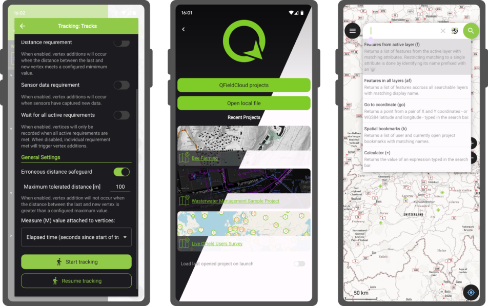
 QField, developed by OPENGIS.ch, is an advanced open-source mobile application that enables GIS professionals to work efficiently in the field, using interactive maps, collecting real-time data, and managing complex geospatial projects on Android, iOS, or Windows mobile devices.
 QField is cross-platform, based on the QGIS engine, facilitating seamless project sharing between desktop, mobile, and web applications.
 QFieldCloud (
 At Oslandia, we are thrilled to collaborate with OPENGIS.ch on QGIS technologies. Oslandia shares with OPENGIS.ch a common vision of open-source software development: a strong involvement in development communities, work in respect with the ecosystem, an highly skilled expertise, and a commitment to industrial-quality, robust, and sustainable software development.
 With this partnership, we aim to offer our clients the highest expertise across all software components of the QGIS platform, from data capture to dissemination.
 On the OpenGIS.ch side, Marco Bernasocchi adds:
 Both companies are committed to continue supporting and improving QField and QFieldCloud as open-source projects, ensuring universal access to this high-quality mobile GIS solution without vendor dependencies.
 And now, are you ready for the field?
 If you need training, support, maintenance, deployment, or specific feature development on these platforms, don’t hesitate to contact us. You will have access to the best experts available:
 You will probably interact first with our pre-sales engineer Bertrand Parpoil. He leads Geographical Information System projects for 15 years for large corporations, public administrations or hi-tech SME. Bertrand will listen to your needs and explore your use cases, to offer you the best set of services.
  Régis Haubourg also takes part in the first steps of projects to analyze your usages and improve them. GIS Expert, he knows QGIS by heart and will make the most of its capabilities. As QGIS Community Manager at Oslandia, he is very active in the QGIS community of developers and contributors. He is president of the Francophone OSGeo local chapter ( OSGeo-fr ), QGIS voting member, organizes the French QGIS day conference in Montpellier, and participates to QGIS community meetings. Before joining Oslandia, he led the migration to QGIS and PostGIS at the Adour-Garonne Water Agency, and now guides our clients with their GIS migrations to OpenSource solutions. Régis is also a great asset when working on water, hydrology and other specific thematic subjects.
 Loïc Bartoletti develops QGIS, specializing in features corresponding to his fields of interests : network management, topography, urbanism, architecture… We find him contributing to advanced vector editing in QGIS, writing Python plugins, namely for DICT management. Pushing CAD and migrations from CAD tools to GIS and QGIS is one of his major goals. He will develop your custom applications, combining technical expertise and functional competences. When bored, Loïc packages software on FreeBSD.
 Vincent Mora is senior developer in Python and C++, as well as PostGIS expert. He has a strong experience in numerical simulation. He likes coupling GIS (PostGIS, QGIS) with 3D numerical computing for risk management or production optimization. Vincent is an official QGIS committer and can directly integrate your needs into the core of the software. He is also GDAL committer and optimizes low-level layers of your applications. Among numerous activities, Vincent serves as lead developer of the development team for
 Hugo Mercier is an officiel QGIS committer too for several years. He regularly talks in international conferences on PostGIS, QGIS and other OpenSource GIS softwares. He will implement your needs with new QGIS features, develop innovative plugins ( like
 Paul Blottière completes our QGIS committers : very active on core development, Paul has refactored the QGIS server component to bring it to an industry-grade quality level. He also designed and implemented
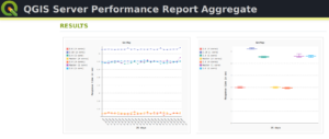
 Julien Cabièces recently joined Oslandia, and quickly dived into QGIS : he contributes to the core of this Desktop GIS, on the server component, as well as applications linked to numerical simulation. Coming from a satellite imagery company with industrial applications, he uses his flexibility to answer all your needs. He brings quality and professionalism to your projects, minimizing risks for large production deployments.
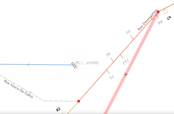
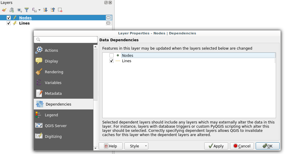 Dependencies configuration: Lines layer will be refreshed whenever Nodes layer is modified
 Snap indexing dialog
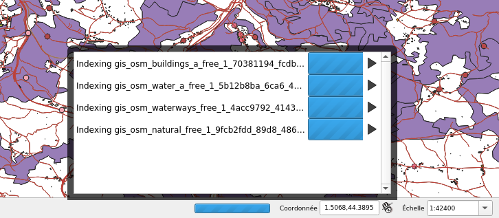 4 layers snap index being built in parallel