
3.1.2 - Borneo
Changes
✨ Improvements
- Update Sentry SDK to increase app stability.
Last update:
Fri Apr 19 04:20:04 2024
 •
•
 •
•

 •
•
 •
•

Previously, we mapped neo4j spatial nodes. This time, we want to take it one step further and map relationships.
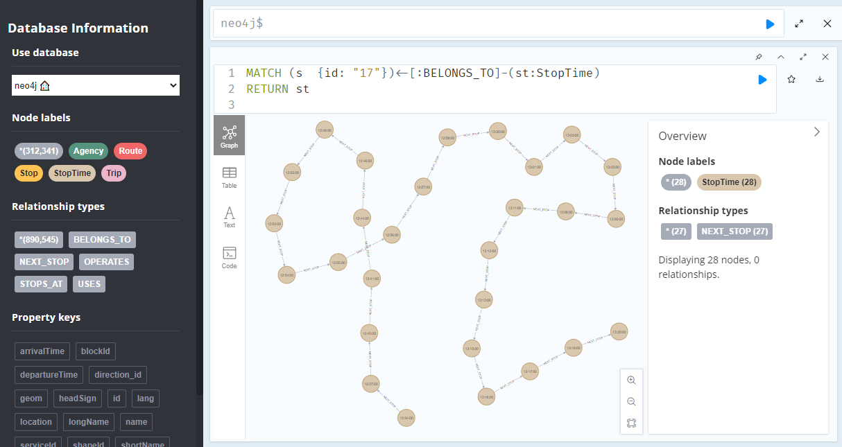
A prime example, are the relationships between GTFS StopTime and Trip nodes. For example, this is the Cypher query to get all StopTime nodes of Trip 17:
MATCH
    (t:Trip  {id: "17"})
    <-[:BELONGS_TO]-
    (st:StopTime)
RETURN st
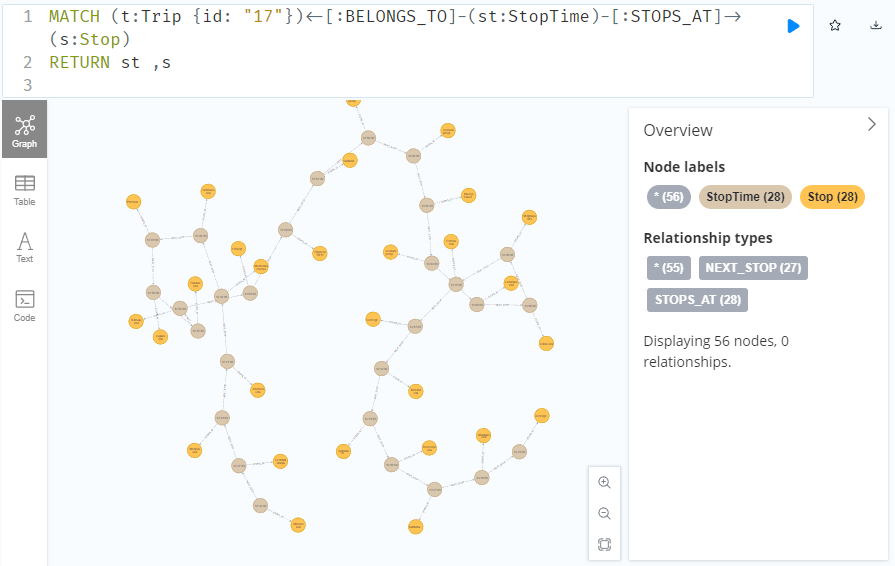
To get the stop locations, we also need to get the stop nodes:
MATCH
    (t:Trip {id: "17"})
    <-[:BELONGS_TO]-
    (st:StopTime)
    -[:STOPS_AT]->
    (s:Stop)
RETURN st ,s
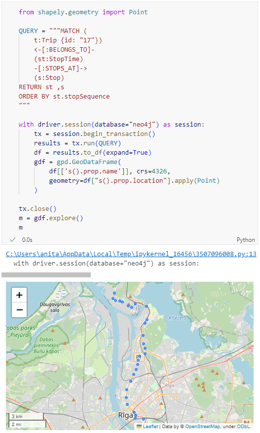
Adapting our code from the previous post, we can plot the stops:
from shapely.geometry import Point

QUERY = """MATCH (
    t:Trip {id: "17"})
    <-[:BELONGS_TO]-
    (st:StopTime)
    -[:STOPS_AT]->
    (s:Stop)
RETURN st ,s
ORDER BY st.stopSequence
"""

with driver.session(database="neo4j") as session:
    tx = session.begin_transaction()
    results = tx.run(QUERY)
    df = results.to_df(expand=True)
    gdf = gpd.GeoDataFrame(
        df[['s().prop.name']], crs=4326,
        geometry=df["s().prop.location"].apply(Point)
    )

tx.close()
m = gdf.explore()
m
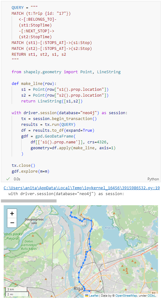
Ordering by stop sequence is actually completely optional. Technically, we could use the sorted GeoDataFrame, and aggregate all the points into a linestring to plot the route. But I want to try something different: we’ll use the NEXT_STOP relationships to get a DataFrame of the start and end stops for each segment:
QUERY = """
MATCH (t:Trip {id: "17"})
   <-[:BELONGS_TO]-
   (st1:StopTime)
   -[:NEXT_STOP]->
   (st2:StopTime)
MATCH (st1)-[:STOPS_AT]->(s1:Stop)
MATCH (st2)-[:STOPS_AT]->(s2:Stop)
RETURN st1, st2, s1, s2
"""

from shapely.geometry import Point, LineString

def make_line(row):
    s1 = Point(row["s1().prop.location"])
    s2 = Point(row["s2().prop.location"])
    return LineString([s1,s2])

with driver.session(database="neo4j") as session:
    tx = session.begin_transaction()
    results = tx.run(QUERY)
    df = results.to_df(expand=True)
    gdf = gpd.GeoDataFrame(
        df[['s1().prop.name']], crs=4326,
        geometry=df.apply(make_line, axis=1)
    )

tx.close()
gdf.explore(m=m)
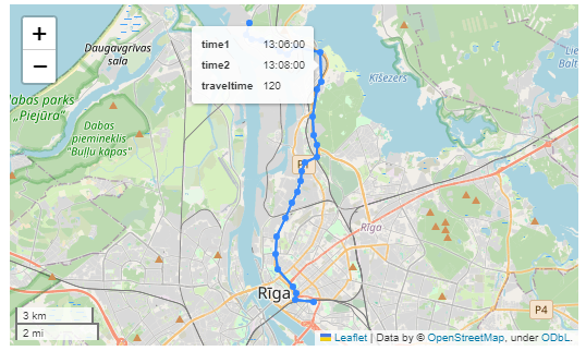
Finally, we can also use Cypher to calculate the travel time between two stops:
MATCH (t:Trip {id: "17"})
   <-[:BELONGS_TO]-
   (st1:StopTime)
   -[:NEXT_STOP]->
   (st2:StopTime)
MATCH (st1)-[:STOPS_AT]->(s1:Stop)
MATCH (st2)-[:STOPS_AT]->(s2:Stop)
RETURN st1.departureTime AS time1,
   st2.arrivalTime AS time2,
   s1.location AS geom1,
   s2.location AS geom2,
   duration.inSeconds(
      time(st1.departureTime),
      time(st2.arrivalTime)
   ).seconds AS traveltime
As always, here’s the notebook: https://github.com/anitagraser/QGIS-resources/blob/master/qgis3/notebooks/neo4j.ipynb
In the recent post Setting up a graph db using GTFS data & Neo4J, we noted that — unfortunately — Neomap is not an option to visualize spatial nodes anymore.
GeoPandas to the rescue!
But first we need the neo4j Python driver:
pip install neo4j
Then we can connect to our database. The default user name is neo4j and you get to pick the password when creating the database:
from neo4j import GraphDatabase

URI = "neo4j://localhost"
AUTH = ("neo4j", "password")

with GraphDatabase.driver(URI, auth=AUTH) as driver:
    driver.verify_connectivity()
Once we have confirmed that the connection works as expected, we can run a query:
QUERY = "MATCH (p:Stop) RETURN p.name AS name, p.location AS geom"

records, summary, keys = driver.execute_query(
    QUERY, database_="neo4j",
)

for rec in records:
    print(rec)
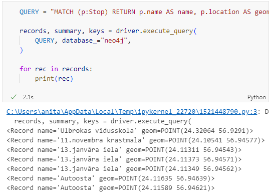
Nice. There we have our GTFS stops, their names and their locations. But how to put them on a map?
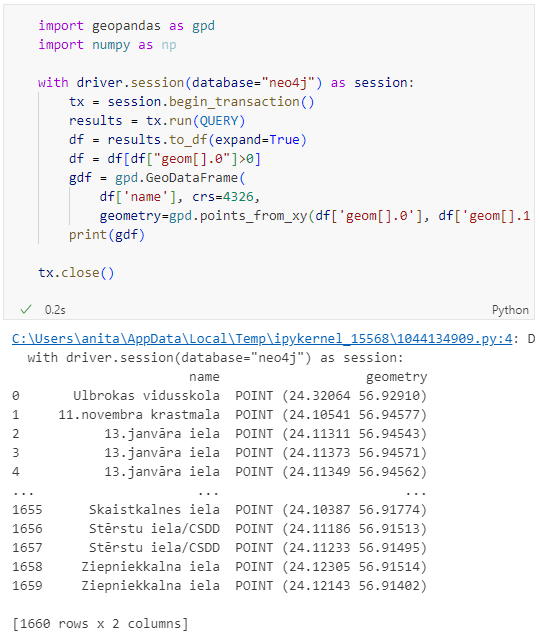
Conveniently, there is a to_db() function in the Neo4j driver:
import geopandas as gpd
import numpy as np

with driver.session(database="neo4j") as session:
    tx = session.begin_transaction()
    results = tx.run(QUERY)
    df = results.to_df(expand=True)
    df = df[df["geom[].0"]>0]
    gdf = gpd.GeoDataFrame(
        df['name'], crs=4326,
        geometry=gpd.points_from_xy(df['geom[].0'], df['geom[].1']))
    print(gdf)

tx.close()
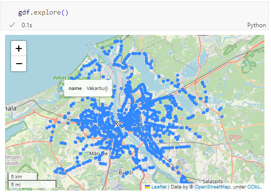
Since some of the nodes lack geometries, I added a quick and dirty hack to get rid of these nodes because — otherwise — gdf.explore() will complain about None geometries.
You can find this notebook at: https://github.com/anitagraser/QGIS-resources/blob/1e4ea435c9b1795ba5b170ddb176aa83689112eb/qgis3/notebooks/neo4j.ipynb
Next step will have to be the relationships. Stay posted.
This autumn, from September to November, 84 new plugins have been published in the QGIS plugin repository.
Here’s the quick overview in reverse chronological order. If any of the names or short descriptions piques your interest, you can find the direct link to the plugin page in the table below:
| SOSIexpressions |
| Expressions related to SOSI-data |
| Puentes |
| Run external Python files inside QGIS. |
| UA CRS Magic |
| Підбір системи кординат для векторного шару |
| FilterMate |
| FilterMate is a Qgis plugin, a daily companion that allows you to easily explore, filter and export vector data |
| QWC2_Tools |
| QGIS plug-in designed to publish and manage the publication of projects in a QWC2 instance. The plugin allows you to publish projects, delete projects and view the list of published projects. |
| QGIS Fast Grid Inspection (FGI) |
| This plugin aims to allow the generation and classification of samples from predefined regions. |
| QDuckDB |
| This plugin adds a new data prodivder that can read DuckDB databases and display their tables as a layer in QGIS. |
| CIGeoE Toggle Label Visibility |
| Toggle label visibility |
| CIGeoE Merge Areas |
| Centro de Informação Geoespacial do Exército |
| Drainage |
| the hydro DEM analysis with the TauDEM |
| Postcode Finder |
| The plugin prompts the user to select the LLPG data layer from the Layers Panel and enter a postcode. The plugin will search for the postcode, if found, the canvas will zoom to all the LLPG points in the postcode. |
| Multi Union |
| This plugin runs the UNION MULTIPLE tool, allowing you to use up to 6 polygon vector layers simultaneously. |
| FLO-2D MapCrafter |
| This plugin creates maps from FLO-2D output files. |
| Download raster GEE |
| download_raster_gee |
| GisCarta |
| Manage your GisCarta data |
| TENGUNGUN |
| To list up and download point cloud data such as “VIRTUAL SHIZUOKA” |
| LADM COL UV |
| Plugin de Qgis para la evaluación de calidad en el proceso de captura y mantenimiento de datos conformes con el modelo LADM-COL |
| ohsomeTools |
| ohsome API, spatial and temporal OSM requests for QGIS |
| Social Burden Calculator |
| This plugin calculates social burden |
| Show Random Changelog Entry on Launch |
| Shows a random entry in the QGIS version’s visual changelog upon QGIS launch |
| Fotowoltaika LP |
| Wyznaczanie lokalizacji pod farmy fotowoltaiczne LP |
| KICa – KAN Imagery Catalog |
| KICa, is QGIS plugin Kan Imagery Catalog, developed by Kan Territory & IT to consult availability of images in an area in an agnostic way, having as main objective to solve the need and not to focus on suppliers. In the beginning, satellite imagery providers (free and commercial) are incorporated, but it is planned to incorporate drone imagery among others. |
| Risk Assessment |
| Risk assessment calculation for forecast based financing |
| ViewDrone |
| A QGIS plugin for viewshed analysis in drone mission planning |
| qgis2opengis |
| Make Lite version of OpenGIS – open source webgis |
| Quick Shape Update |
| Automatic update of the shapes length and/or area in the selected layer |
| CoolParksTool |
| This plugin evaluates the cooling effect of a park and its impact on buildings energy and thermal comfort |
| Nahlížení do KN |
| Unofficial integration for Nahlížení do Katastru nemovitostí. |
| PyGeoRS |
| PyGeoRS is a dynamic QGIS plugin designed to streamline and enhance your remote sensing workflow within the QGIS environment. |
| D4C Plugin |
| This plugin allows the manbipulation from QGis of Data4Citizen datasets (Open Data platform based on Drupal and CKan) |
| Avenza Maps’s KML/KMZ File Importer |
| This plugin import features from KML e KMZ files from Avenza Maps |
| Histogram Matching |
| Image histogram matching process |
| PV Prospector |
| Displays the PV installation potential for residential properties. The pv_area layer is derived from 1m LIDAR DSM, OSMM building outlines and LLPG data. |
| Save Attributes (Processing) |
| This plugin adds an algorithm to save attributes of selected layer as a CSV file |
| Artificial Intelligence Forecasting Remote Sensing |
| This plugin allows time series forecasting using deep learning models. |
| Salvar Pontos TXT |
| Esse plugin salvar camada de pontos em arquivo TXT |
| QGIS to Illustrator with PlugX |
| The plugin to convert QGIS maps to import from Illustrator. With PlugiX-QGIS, you can transfer maps designed in QGIS to Illustrator! |
| QCrocoFlow |
| A QGIS plugin to manage CROCO projectsqcrocoflow |
| Soft Queries |
| This plugin brings tools that allow processing of data using fuzzy set theory and possibility theory. |
| TerrainZones |
| This Plugin Identifies & Creates Sub-Irrigation Zones |
| Consolidate Networks |
| Consolidate Networks is a a Qgis plugin bringing together a set of tools to consolidate your network data. |
| AWD |
| Automatic waterfalls detector |
| SAGis XPlanung |
| Plugin zur XPlanung-konformen Erfassung und Verwaltung von Bauleitplänen |
| Monitask |
| a SAM (facebook segment anything model and its decendants) based geographic information extraction tool just by interactive click on remote sensing image, as well as an efficient geospatial labeling tool. |
| PLATEAU QGIS Plugin |
| Import the PLATEAU 3D City Models (CityGML) used in Japan — PLATEAU 3D都市モデルのCityGMLファイルをQGISに読み込みます |
| FLO-2D Rasterizor |
| A plugin to rasterize general FLO-2D output files. |
| Geoportal Lokalizator |
| PL: Wtyczka otwiera rządowy geoportal w tej samej lokacji w której użytkownik ma otwarty canvas QGIS-a. EN: The plugin opens the government geoportal in the same location where the user has the QGIS canvas open (Poland only). |
| BorderFocus |
| clicks on the edge center them on the canvas |
| LANDFILL SITE SELECTION |
| LANDFILL SITE SELECTION |
| Bearing & Distance |
| This plugin contains tools for the calculation of bearing and distances for both single and multiple parcels. |
| Moisture and Water Index 2.0 |
| Este complemento calcula el índice NDWI con las imágenes del Landsat 8. |
| K-L8Slice |
| Este nombre combina el algoritmo k-means que se utiliza para el agrupamiento (K) con “Landsat 8”, que es el tipo específico de imágenes satelitales utilizadas, y “Slicer”, que hace referencia al proceso de segmentación o corte de la imagen en diferentes clusters o grupos de uso del suelo. |
| EcoVisioL8 |
| Este complemento fue diseñado para automatizar y optimizar la obtención de índices SAVI, NDVI y SIPI, así como la realización de correcciones atmosféricas en imágenes Landsat 8. |
| QGIS Animation Workbench |
| A plugin to let you build animations in QGIS |
| Catastro con Historia |
| Herramienta para visualizar el WMS de Catastro en pantalla partida con historia. |
| RechercheCommune |
| Déplace la vue sur l’emprise de la commune choisie. |
| Sentinel2 SoloBand |
| Sentinel2 SoloBand is a plugin for easily searching for individual bands in Sentinel-2 imagery. |
| CIGeoE Right Angled Symbol Rotation |
| Right Angled Symbol Rotation |
| CIGeoE Node Tool |
| Tool to perform operations over nodes of a selected feature, not provided by similar tools and plugins. |
| Spatial Distribution Pattern |
| This plugin estimates the Spatial Distribution Pattern of point and linear features. |
| Webmap Utilities |
| This plugin provides tools for clustered and hierarchical visualization of vector layers, creation of Relief Shading and management of scales using zoom levels. |
| Simstock QGIS |
| Allows urban building energy models to be created and simulated within QGIS |
| Fast Point Inspection |
| Fast Point Inspection is a QGIS plugin that streamlines the process of classifying point geometries in a layer. |
| Layer Grid View |
| The Layer Grid Plugin provides an intuitive dockable widget that presents a grid of map canvases. |
| Kadastr.Live Toolbar |
| Пошук ділянки на карті Kadastr.Live за кадастровим номером. |
| S+HydPower |
| Plugin designed to estimate hydropower generation. |
| QollabEO |
| Collaborative functions for interaction with remote users. |
| digitizer |
| digitizer |
| NetADS |
| NetADS est un logiciel web destiné à l’instruction dématérialisée des dossiers d’urbanisme. |
| Runoff Model: RORB |
| Build a RORB control vector from a catchment |
| FlexGIS |
| Manage your FlexGIS data |
| LXExportDistrict |
| Export administrative district |
| PostGIS Toolbox |
| Plugin for QGIS implementing selected PostGIS functions |
| Chasse – Gestion des lots |
| Fonctions permettant de définir la surface cadastrale des lots de chasse et d’extraire la liste des parcelles concernées par chaque lot de chasse, sous forme de fichier Excel®. |
| Time Editor |
| Used to facilitate the editing of features with lifespan information |
| RST |
| This plugin computes biophysical indices |
| Japanese Grid Mesh |
| Create common grid squares used in Japan. 日本で使われている「標準地域メッシュ」および「国土基本図図郭」を作成できます。また、国勢調査や経済センサスなどの「地域メッシュ統計」のCSVファイルを読み込むこともできます。プロセッシングツールボックスから利用できます。 |
| Panoramax |
| Upload, load and display your immersive views hosted on a Panoramax instance. |
| StereoPhoto |
| Permet la visualisation d’images avec un système stéréoscopique |
| CIGeoE Merge Multiple Lines |
| Merge multiple lines by coincident vertices and with the same attribute names and values. |
| CIGeoE Merge Lines |
| Merge 2 lines that overlap (connected in a vertex) and have same attribute names and values. |
| Nimbo’s Earth Basemaps |
| Nimbo’s Earth Basemaps is an innovative Earth observation service providing cloud-free, homogenous mosaics of the world’s entire landmass as captured by satellite imagery, updated every month. |
| OpenHLZ |
| An Open-source HLZ Identification Processing Plugin |
| Selection as Filter |
| This plugin makes filter for the selected features |
Today, I want to point out a blog post over at
https://carto.com/blog/analyzing-mobility-hotspots-with-movingpandas
written together with my fellow co-authors and EMERALDS project team members Argyrios Kyrgiazos and Helen McKenzie.
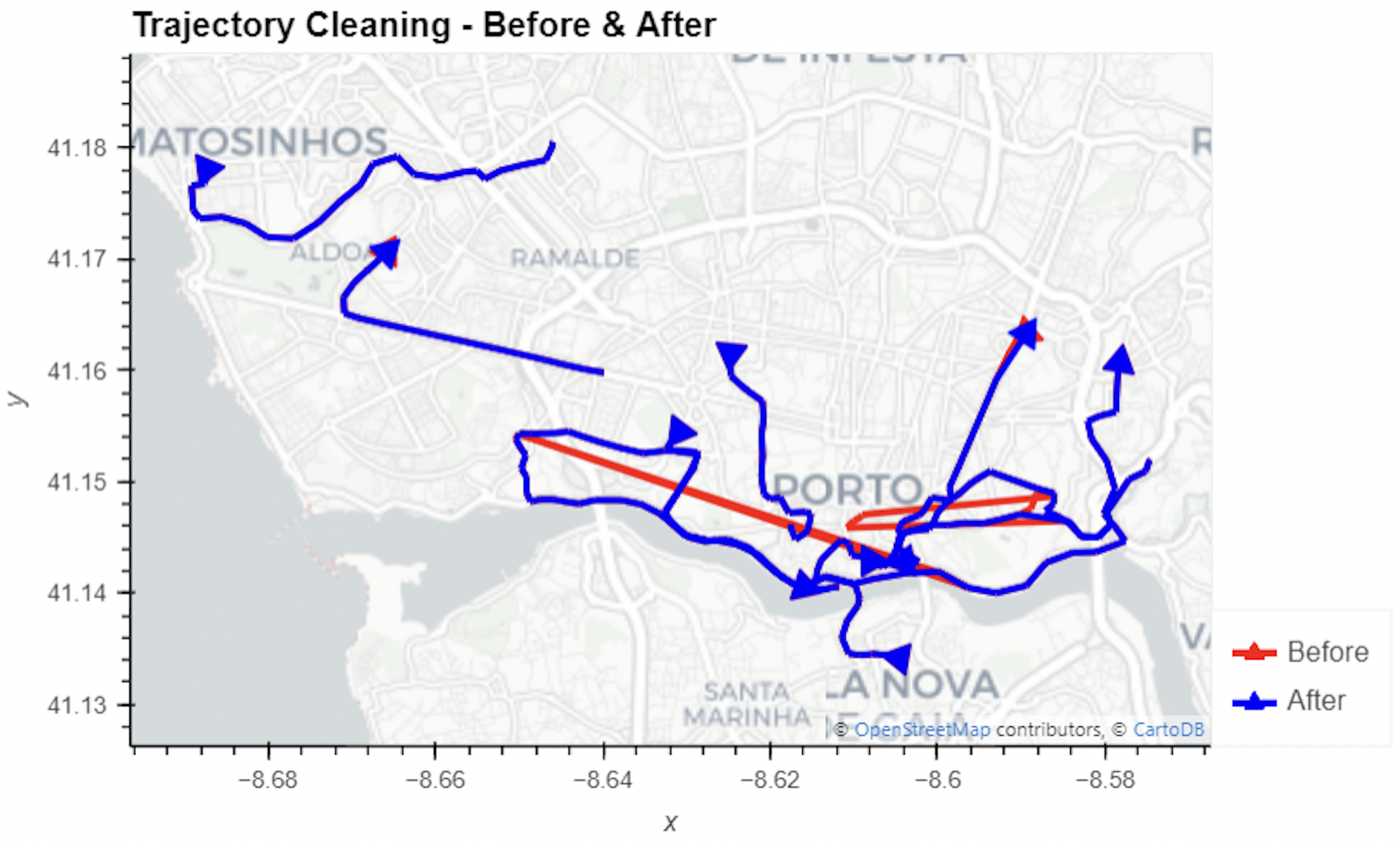
In this blog post, we walk you through a trajectory hotspot analysis using open taxi trajectory data from Kaggle, combining data preparation with MovingPandas (including the new OutlierCleaner illustrated above) and spatiotemporal hotspot analysis from Carto.
In a recent post, we looked into a graph-based model for maritime mobility data and how it may be represented in Neo4J. Today, I want to look into another type of mobility data: public transport schedules in GTFS format.
In this post, I’ll be using the public GTFS data for Riga since Riga is one of the demo sites for our current EMERALDS research project.
The workflow is heavily inspired by Bert Radke‘s post “Loading the UK GTFS data feed” from 2021 and his import Cypher script which I used as a template, adjusted to the requirements of the Riga dataset, and updated to recent Neo4J changes.
Here we go.
Since a GTFS export is basically a ZIP archive full of CSVs, we will be making good use of Neo4Js CSV loading capabilities. The basic script for importing the stops file and creating point geometries from lat and lon values would be:
LOAD CSV with headers
FROM "file:///stops.txt"
AS row
CREATE (:Stop {
   stop_id: row["stop_id"],
   name: row["stop_name"],
   location: point({
    longitude: toFloat(row["stop_lon"]),
    latitude: toFloat(row["stop_lat"])
    })
})
This requires that the stops.txt is located in the import directory of your Neo4J database. When we run the above script and the file is missing, Neo4J will tell us where it tried to look for it. In my case, the directory ended up being:
C:\Users\Anita\.Neo4jDesktop\relate-data\dbmss\dbms-72882d24-bf91-4031-84e9-abd24624b760\import
So, let’s put all GTFS CSVs into that directory and we should be good to go.
Let’s start with the agency file:
load csv with headers from
'file:///agency.txt' as row
create (a:Agency {
   id: row.agency_id,
   name: row.agency_name,
   url: row.agency_url,
   timezone: row.agency_timezone,
   lang: row.agency_lang
});
… Added 1 label, created 1 node, set 5 properties, completed after 31 ms.
The routes file does not include agency info but, luckily, there is only one agency, so we can hard-code it:
load csv with headers from
'file:///routes.txt' as row
match (a:Agency {id: "rigassatiksme"})
create (a)-[:OPERATES]->(r:Route {
   id: row.route_id,
   shortName: row.route_short_name,
   longName: row.route_long_name,
   type: toInteger(row.route_type)
});
… Added 81 labels, created 81 nodes, set 324 properties, created 81 relationships, completed after 28 ms.
From stops, I’m removing non-existent or empty columns:
load csv with headers from
'file:///stops.txt' as row
create (s:Stop {
   id: row.stop_id,
   name: row.stop_name,
   location: point({
      latitude: toFloat(row.stop_lat),
      longitude: toFloat(row.stop_lon)
   }),
   code: row.stop_code
});
… Added 1671 labels, created 1671 nodes, set 5013 properties, completed after 71 ms.
From trips, I’m also removing non-existent or empty columns:
load csv with headers from
'file:///trips.txt' as row
match (r:Route {id: row.route_id})
create (r)<-[:USES]-(t:Trip {
   id: row.trip_id,
   serviceId: row.service_id,
   headSign: row.trip_headsign,
   direction_id: toInteger(row.direction_id),
   blockId: row.block_id,
   shapeId: row.shape_id
});
… Added 14427 labels, created 14427 nodes, set 86562 properties, created 14427 relationships, completed after 875 ms.
Slowly getting there. We now have around 16k nodes in our graph:
Finally, it’s stop times time. This is where the serious information is. This file is much larger than all previous ones with over 300k lines (i.e. times when an PT vehicle stops).
This requires another tweak to Bert’s script since using periodic commit is not supported anymore: The PERIODIC COMMIT query hint is no longer supported. Please use CALL { … } IN TRANSACTIONS instead. So I ended up using the following, based on https://community.neo4j.com/t/best-practice-for-replacement-of-using-periodic-commit-to-call-in-transactions/48636/2:
:auto
load csv with headers from
'file:///stop_times.txt' as row
CALL { with row
match (t:Trip {id: row.trip_id}), (s:Stop {id: row.stop_id})
create (t)<-[:BELONGS_TO]-(st:StopTime {
   arrivalTime: row.arrival_time,
   departureTime: row.departure_time,
   stopSequence: toInteger(row.stop_sequence)})-[:STOPS_AT]->(s)
} IN TRANSACTIONS OF 10 ROWS;
… Added 351388 labels, created 351388 nodes, set 1054164 properties, created 702776 relationships, completed after 1364220 ms.
As you can see, this took a while. But now we have all nodes in place:


The final statement adds additional relationships between consecutive stop times:
call apoc.periodic.iterate('match (t:Trip) return t',
'match (t)<-[:BELONGS_TO]-(st) with st order by st.stopSequence asc
with collect(st) as stops
unwind range(0, size(stops)-2) as i
with stops[i] as curr, stops[i+1] as next
merge (curr)-[:NEXT_STOP]->(next)', {batchmode: "BATCH", parallel:true, parallel:true, batchSize:1});
This fails with: There is no procedure with the name apoc.periodic.iterate registered for this database instance. Please ensure you've spelled the procedure name correctly and that the procedure is properly deployed.
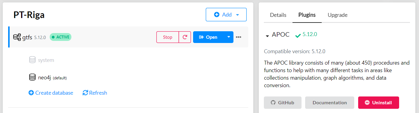
So, let’s install APOC. That’s a plugin which we can install into our database from within Neo4J Desktop:
After restarting the db, we can run the query:
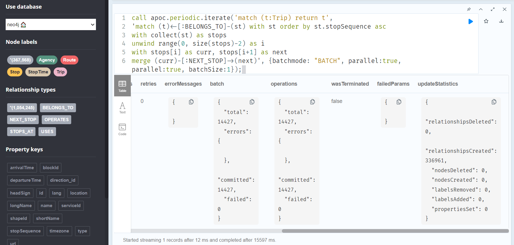
No errors. Sounds good.
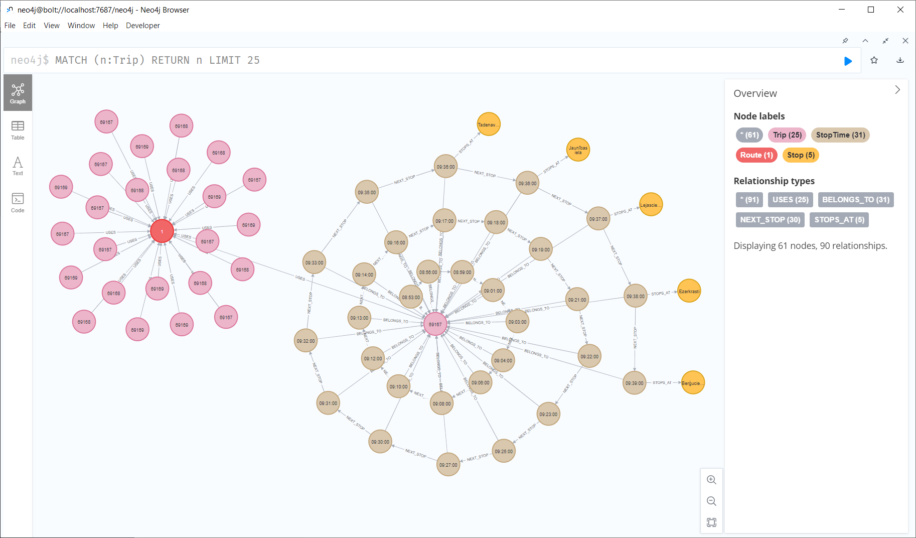
Let’s have a look at what we ended up with. Here are 25 random Trips. I expanded one of them to show its associated StopTimes. We can see the relations between consecutive StopTimes and I’ve expanded the final five StopTimes to show their linked Stops:
I also wanted to visualize the stops on a map. And there used to be a neat app called Neomap which can be installed easily:

However, Neomap does not seem to be compatible with the latest Neo4J:

So this final step will have to wait for another time.
Very simple way of how to display map service in QGI3 without a map server.
Details of MapTiler QGIS Plugin 3.0 with a global terrain basemap and customizable OpenStreetMap vector tiles.
Open-source plugin for QGIS that loads fast vector maps. Change colors and fonts of the map to get unique look.
The new version of the MapTiler plugin pushes our maps from MapTiler Cloud almost to perfection
The new QGIS 3.14 version adds support for the native loading of vector tiles. The easiest way to load them is via the recently released plugin.
Full Changelog: v3.0.6...v3.0.7
Earlier this year, in collaboration with North Road we were awarded a grant from Cesium to introduce 3D tiles support in QGIS. The feature was developed successfully and shipped with QGIS 3.34.
In this blog post, you can read more about how to work with this feature, where to get data and how to display your maps in 2D and 3D. For a video demo of this feature, you can watch Nyall Dawson’s presentation on Youtube.
3D tiles are a specification for streaming and rendering large-scale 3D geospatial datasets. They use a hierarchical structure to efficiently manage and display 3D content, optimising performance by dynamically loading appropriate levels of detail. This technology is widely used in urban planning, architecture, simulation, gaming, and virtual reality, providing a standardised and interoperable solution for visualising complex geographical data.
Examples of 3D tiles:

")
To be able to use 3D tiles in QGIS, you need to have QGIS 3.34 or later. You can add a new connection to a 3D tile service from within the Data Source Manager under Scene:

Alternatively, you can add the service from your Browser Panel:

To test the feature, you can use the following 3D tiles service:
Name: 3D Tiles example
URL: https://pelican-public.s3.amazonaws.com/3dtiles/agi-hq/tileset.json

You can then add the map from the newly generated connection to QGIS:

By default, the layer is styled using texture, but you can change it to see the wireframe mesh behind the scene:

You can change the mesh fill and line symbols similar to the vector polygons. Alternatively, you can use texture colors. This will render each mesh element with the average value of the full texture. This is ideal when dealing with a large dataset and want to get a quick overview of the data:

To view the data in 3D, you can open a new 3D map. Similar to 2D map, by zooming in/out, finer resolution tiles will be fetched and displayed:
Cesium ion is a cloud-based platform for managing and streaming 3D geospatial data. It simplifies data management, visualisation, and sharing.
To add 3D tiles from Cesium ion, you need to first sign up to their service here: https://ion.cesium.com/tokens
Under Asset Depot, you will see a catalogue of publicly available datasets. You can also upload your own 3D models (such as OBJ or PLY), georeference them and get them converted to 3D tiles.
You can also add one of the existing tile service under https://ion.cesium.com/assetdepot and select the tile service and then click on Add to my assets:

You can use the excellent Cesium ion plugin by North Road from the QGIS repository to add the data to QGIS:

In addition to accessing Google Photorealistic 3D tiles from Cesium ion, you can also add the tiles directly in QGIS. First you will need to follow the instructions below and obtain API keys for 3D tiles: https://developers.google.com/maps/documentation/tile/cloud-setup
During the registration process, you will be asked to add your credit card details. Currently (November 2023), they do not charge you for using the service.
Once you have obtained the API key, you can add Google tiles using the following connection details:

When dealing with large scenes, map extents should be set to a smaller area to be able to view it in 3D. This is the current limitation of QGIS 3D maps as it cannot handle scenes larger than 500 x 500 km.
To change the map extent, you can open Project Properties and under View Settings change the extent. In the example below, the map extent has been limited only to a part of London, so we can view Google Photorealistic tiles in the 3D map without rendering issues.


If you are handling a large dataset, it is recommended to increase network cache size to 1 GB or more. The default value in QGIS is much lower and it results in slower rendering of the data.

When you try to overlay other data sets on top of a global 3D tiles, the vertical datum might not match and hence you will see the data in the wrong place in a 3D map. To fix the issue, you may need to use elevation offsetting to shift the data along the Z axis under Layer Properties:

This is the first implementation of the 3D tiles in QGIS. For the future, we would like to add more features for handling and creation of the 3D tiles. Our wishlist in no particular order is:

If you would like to see those features in QGIS and want to fund the efforts, do not hesitate to contact us.
Over the last couple of months, I have not been posting release announcements here, so there is quite a bit to catch up.
The latest v0.17.2 release is now available from conda-forge.
New features (since 0.14):
Behind the scenes:
As always, all tutorials are available from the movingpandas-examples repository and on MyBinder:

If you have questions about using MovingPandas or just want to discuss new ideas, you’re welcome to join our discussion forum.
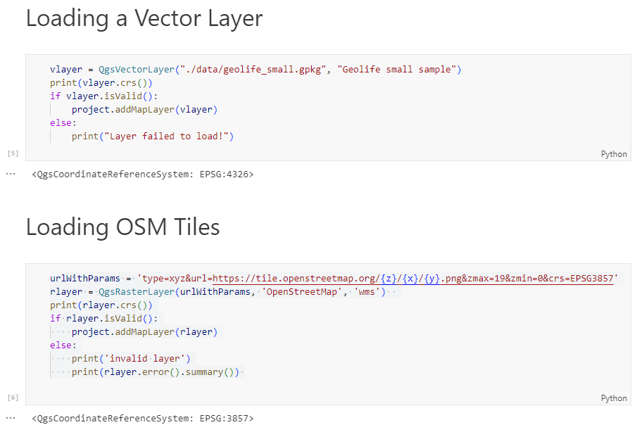
In the previous post, we investigated how to bring QGIS maps into Jupyter notebooks.
Today, we’ll take the next step and add basemaps to our maps. This is trickier than I would have expected. In particular, I was fighting with “invalid” OSM tile layers until I realized that my QGIS application instance somehow lacked the “WMS” provider.
In addition, getting basemaps to work also means that we have to take care of layer and project CRSes and on-the-fly reprojections. So let’s get to work:
from IPython.display import Image
from PyQt5.QtGui import QColor
from PyQt5.QtWidgets import QApplication
from qgis.core import QgsApplication, QgsVectorLayer, QgsProject, QgsRasterLayer, \
    QgsCoordinateReferenceSystem, QgsProviderRegistry, QgsSimpleMarkerSymbolLayerBase
from qgis.gui import QgsMapCanvas
app = QApplication([])
qgs = QgsApplication([], False)
qgs.setPrefixPath(r"C:\temp", True)  # setting a prefix path should enable the WMS provider
qgs.initQgis()
canvas = QgsMapCanvas()
project = QgsProject.instance()
map_crs = QgsCoordinateReferenceSystem('EPSG:3857')
canvas.setDestinationCrs(map_crs)
print("providers: ", QgsProviderRegistry.instance().providerList())

To add an OSM basemap, we use the xyz tiles option of the WMS provider:
urlWithParams = 'type=xyz&url=https://tile.openstreetmap.org/{z}/{x}/{y}.png&zmax=19&zmin=0&crs=EPSG3857'
rlayer = QgsRasterLayer(urlWithParams, 'OpenStreetMap', 'wms')
print(rlayer.crs())
if rlayer.isValid():
    project.addMapLayer(rlayer)
else:
    print('invalid layer')
    print(rlayer.error().summary())
If there are issues with the WMS provider, rlayer.error().summary() should point them out.
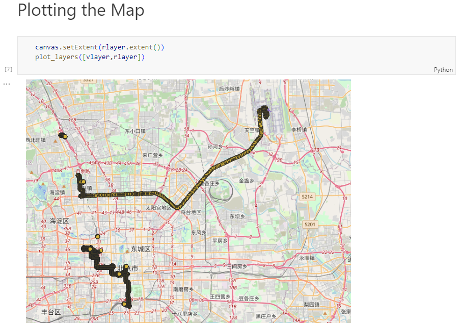
With both the vector layer and the basemap ready, we can finally plot the map:
canvas.setExtent(rlayer.extent())
plot_layers([vlayer,rlayer])
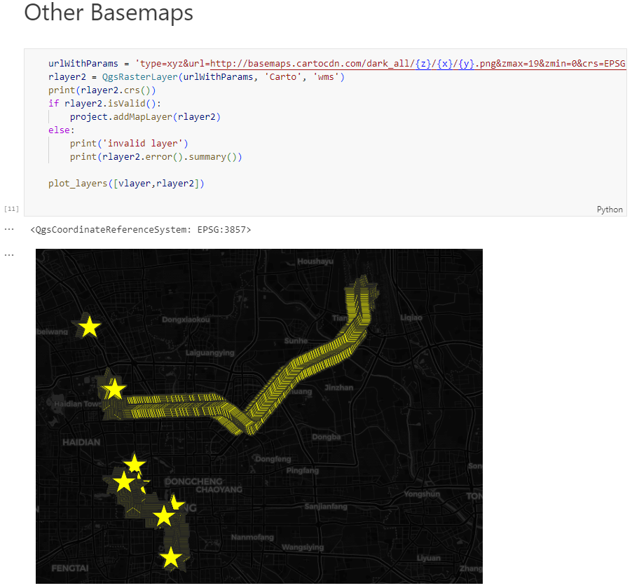
Of course, we can get more creative and style our vector layers:
vlayer.renderer().symbol().setColor(QColor("yellow"))
vlayer.renderer().symbol().symbolLayer(0).setShape(QgsSimpleMarkerSymbolLayerBase.Star)
vlayer.renderer().symbol().symbolLayer(0).setSize(10)
plot_layers([vlayer,rlayer])

And to switch to other basemaps, we just need to update the URL accordingly, for example, to load Carto tiles instead:
urlWithParams = 'type=xyz&url=http://basemaps.cartocdn.com/dark_all/{z}/{x}/{y}.png&zmax=19&zmin=0&crs=EPSG3857'
rlayer2 = QgsRasterLayer(urlWithParams, 'Carto', 'wms')
print(rlayer2.crs())
if rlayer2.isValid():
    project.addMapLayer(rlayer2)
else:
    print('invalid layer')
    print(rlayer2.error().summary())

plot_layers([vlayer,rlayer2])
You can find the whole notebook at: https://github.com/anitagraser/QGIS-resources/blob/master/qgis3/notebooks/basemaps.ipynb
Open source software projects thrive on the contributions of the community, not only for the code, but also for making the software accessible to a global audience. One of the critical aspects of this accessibility is the localization or translation of the software’s messages and interfaces. In this context, Weblate (https://weblate.org/) has proven to be […]
The post Translating Open Source Software with Weblate: A GRASS GIS Case Study appeared first on Markus Neteler Consulting.
Earlier this year, we explored how to use PyQGIS in Juypter notebooks to run QGIS Processing tools from a notebook and visualize the Processing results using GeoPandas plots.
Today, we’ll go a step further and replace the GeoPandas plots with maps rendered by QGIS.
The following script presents a minimum solution to this challenge: initializing a QGIS application, canvas, and project; then loading a GeoJSON and displaying it:
from IPython.display import Image

from PyQt5.QtGui import QColor
from PyQt5.QtWidgets import QApplication

from qgis.core import QgsApplication, QgsVectorLayer, QgsProject, QgsSymbol, \
    QgsRendererRange, QgsGraduatedSymbolRenderer, \
    QgsArrowSymbolLayer, QgsLineSymbol, QgsSingleSymbolRenderer, \
    QgsSymbolLayer, QgsProperty
from qgis.gui import QgsMapCanvas

app = QApplication([])
qgs = QgsApplication([], False)
canvas = QgsMapCanvas()
project = QgsProject.instance()

vlayer = QgsVectorLayer("./data/traj.geojson", "My trajectory")
if not vlayer.isValid():
    print("Layer failed to load!")

def saveImage(path, show=True):
    canvas.saveAsImage(path)
    if show: return Image(path)

project.addMapLayer(vlayer)
canvas.setExtent(vlayer.extent())
canvas.setLayers([vlayer])
canvas.show()
app.exec_()

saveImage("my-traj.png")
When this code is executed, it opens a separate window that displays the map canvas. And in this window, we can even pan and zoom to adjust the map. The line color, however, is assigned randomly (like when we open a new layer in QGIS):

To specify a specific color, we can use:
vlayer.renderer().symbol().setColor(QColor("red"))

vlayer.triggerRepaint()
canvas.show()
app.exec_()
saveImage("my-traj.png")

But regular lines are boring. We could easily create those with GeoPandas plots.
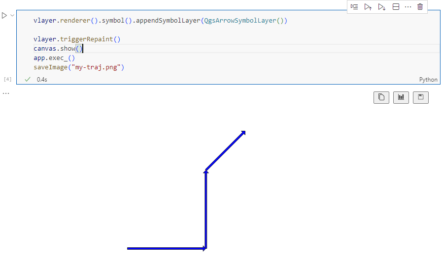
Things get way more interesting when we use QGIS’ custom symbols and renderers. For example, to draw arrows using a QgsArrowSymbolLayer, we can write:
vlayer.renderer().symbol().appendSymbolLayer(QgsArrowSymbolLayer())

vlayer.triggerRepaint()
canvas.show()
app.exec_()
saveImage("my-traj.png")
We can also create a QgsGraduatedSymbolRenderer:
geom_type = vlayer.geometryType()
myRangeList = []

symbol = QgsSymbol.defaultSymbol(geom_type)
symbol.setColor(QColor("#3333ff"))
myRange = QgsRendererRange(0, 1, symbol, 'Group 1')
myRangeList.append(myRange)

symbol = QgsSymbol.defaultSymbol(geom_type)
symbol.setColor(QColor("#33ff33"))
myRange = QgsRendererRange(1, 3, symbol, 'Group 2')
myRangeList.append(myRange)

myRenderer = QgsGraduatedSymbolRenderer('speed', myRangeList)
vlayer.setRenderer(myRenderer)

vlayer.triggerRepaint()
canvas.show()
app.exec_()
saveImage("my-traj.png")

And we can combine both QgsGraduatedSymbolRenderer and QgsArrowSymbolLayer:
geom_type = vlayer.geometryType()
myRangeList = []

symbol = QgsSymbol.defaultSymbol(geom_type)
symbol.appendSymbolLayer(QgsArrowSymbolLayer())
symbol.setColor(QColor("#3333ff"))
myRange = QgsRendererRange(0, 1, symbol, 'Group 1')
myRangeList.append(myRange)

symbol = QgsSymbol.defaultSymbol(geom_type)
symbol.appendSymbolLayer(QgsArrowSymbolLayer())
symbol.setColor(QColor("#33ff33"))
myRange = QgsRendererRange(1, 3, symbol, 'Group 2')
myRangeList.append(myRange)

myRenderer = QgsGraduatedSymbolRenderer('speed', myRangeList)
vlayer.setRenderer(myRenderer)

vlayer.triggerRepaint()
canvas.show()
app.exec_()
saveImage("my-traj.png")

Maybe the most powerful option is to use data-defined symbology. For example, to control line width and color:
renderer = QgsSingleSymbolRenderer(QgsSymbol.defaultSymbol(geom_type))

exp_width = 'scale_linear("speed", 0, 3, 0, 7)'
exp_color = "coalesce(ramp_color('Viridis',scale_linear(\"speed\", 0, 3, 0, 1)), '#000000')"

# https://qgis.org/pyqgis/3.0/core/Symbol/QgsSymbolLayer.html?highlight=property#qgis.core.QgsSymbolLayer.PropertySize
renderer.symbol().symbolLayer(0).setDataDefinedProperty(
    QgsSymbolLayer.PropertyStrokeWidth, QgsProperty.fromExpression(exp_width))
renderer.symbol().symbolLayer(0).setDataDefinedProperty(
    QgsSymbolLayer.PropertyStrokeColor, QgsProperty.fromExpression(exp_color))
renderer.symbol().symbolLayer(0).setDataDefinedProperty(
    QgsSymbolLayer.PropertyCapStyle, QgsProperty.fromExpression("'round'"))

vlayer.setRenderer(renderer)

vlayer.triggerRepaint()
canvas.show()
app.exec_()
saveImage("my-traj.png")

Find the full notebook at: https://github.com/anitagraser/QGIS-resources/blob/master/qgis3/notebooks/layer-styling.ipynb
Sorry, this entry is only available in Dutch.
We’ve recently had the opportunity to implement a very exciting feature in QGIS 3.34 — the ability to load and view 3D content in the “Cesium 3D Tiles” format! This was a joint project with our (very talented!) partners at Lutra Consulting, and was made possible thanks to a generous ecosystem grant from the Cesium project.
Before we dive into all the details, let’s take a quick guided tour showcasing how Cesium 3D Tiles work inside QGIS:
Cesium 3D Tiles are an OGC standard data format where the content from a 3D scene is split up into multiple individual tiles. You can think of them a little like a 3D version of the vector tile format we’ve all come to rely upon. The 3D objects from the scene are stored in a generalized, simplified form for small-scale, “zoomed out” maps, and in more detailed, complex forms for when the map is zoomed in. This allows the scenes to be incredibly detailed, whilst still covering huge geographic regions (including the whole globe!) and remaining responsive and quick to download. Take a look at the incredible level of detail available in a Cesium 3D Tiles scene in the example below:
If you’re lucky, your regional government or data custodians are already publishing 3D “digital twins” of your area. Cesium 3D Tiles are the standard way that these digital twin datasets are being published. Check your regional data portals and government open data hubs and see whether they’ve made any content available as 3D tiles. (For Australian users, there’s tons of great content available on the Terria platform!).
Alternatively, there’s many datasets available via the Cesium ion platform. This includes global 3D buildings based on OpenStreetMap data, and the entirety of Google’s photorealistic Google Earth tiles! We’ve published a Cesium ion QGIS plugin to complement the QGIS 3.34 release, which helps make it super-easy to directly load datasets from ion into your QGIS projects.
Lastly, users of the OpenDroneMap photogrammetry application will already have Cesium 3D Tiles datasets of their projects available, as 3D tiles are one of the standard outputs generated by OpenDroneMap.
So why exactly would you want to access Cesium 3D tiles within QGIS? Well, for a start, 3D Tiles datasets are intrinsically geospatial data. All the 3D content from these datasets are georeferenced and have accurate spatial information present. By loading a 3D tiles dataset into QGIS, you can easily overlay and compare 3D tile content to all your other standard spatial data formats (such as Shapefiles, Geopackages, raster layers, mesh datasets, WMS layers, etc…). They become just another layer of spatial information in your QGIS projects, and you can utilise all the tools and capabilities you’re familiar with in QGIS for analysing spatial data along with these new data sources.
One large drawcard of adding a Cesium 3D Tile dataset to your QGIS project is that they make fantastic 3D basemaps. While QGIS has had good support for 3D maps for a number of years now, it has been tricky to create beautiful 3D content. That’s because all the standard spatial data formats tend to give generalised, “blocky” representations of objects in 3D. For example, you could use an extruded building footprint file to show buildings in a 3D map but they’ll all be colored as idealised solid blocks. In contrast, Cesium 3D Tiles are a perfect fit for a 3D basemap! They typically include photorealistic textures, and include all types of real-world features you’d expect to see in a 3D map — including buildings, trees, bridges, cliffsides, etc.
If you’re keen to learn even more about Cesium 3D Tiles in QGIS, you can check out the recent “QGIS Open Day” session we presented. In this session we cover all the details about 3D tiles and QGIS, and talk in depth about what’s possible in QGIS 3.34 and what may be coming in later releases.
Otherwise, grab the latest QGIS 3.34 and start playing…. you’ll quickly find that Cesium 3D Tiles are a fun and valuable addition to QGIS’ capabilities!
Our thanks go to Cesium and their ecosystem grant project for funding this work and making it possible.
